N-Layer Dyadic Green’s Function Workflow

Goal

This tutorial shows the shortest reproducible path for computing dyadic Green’s functions in a finite planar multilayer stack with mqed_GF_NLayer. Use this solver when the environment is translationally invariant in the horizontal plane, but has more than the two media handled by the basic Sommerfeld tutorial.

By the end you will know how to:

• run the five-layer Ag/spacer example,

• interpret the layer order and emitter coordinates,

• choose between the separation output layout and downstream analyses,

• launch larger frequency sweeps with the SGE/MPI helper script.

When to use this solver

Green-function solver choices

Solver	Geometry	Typical output layout
mqed_GF_Sommerfeld	Two-layer planar interface	separation: one tensor per horizontal distance Rx
mqed_GF_NLayer	Arbitrary planar stack of finite and semi-infinite layers	separation: one tensor per horizontal distance Rx
mqed_GF_Mie	Sphere, spherical cavity, or core-shell sphere	scan for fixed-source scans, or pair for emitter lists

The important point is that the N-layer solver still has horizontal translational symmetry. If two emitter pairs have the same lateral separation Rx and the same vertical positions zD/zA, they reuse the same Green tensor.

Quick run

The bundled wrapper config is:

configs/Dyadic_GF/GF_NLayer_five_layer.yaml

It loads the documented five-layer example in configs/Dyadic_GF/GF_five_layer_example_multi_freq.yaml. Run it with:

mqed_GF_NLayer --config-name GF_NLayer_five_layer

For a quick smoke test before starting the full frequency sweep, override the energy and distance grids from the command line:

mqed_GF_NLayer \
  --config-name GF_NLayer_five_layer \
  parallel.backend=sequential \
  simulation.energy_eV='[1.0]' \
  simulation.position.Rx_nm.start=0 \
  simulation.position.Rx_nm.stop=0 \
  simulation.position.Rx_nm.points=1

The production example writes a file with a name similar to:

NLayer_GF_five_layer_Ag_spacer_Emin_0.10_Emax_6.00_419pts_Rx_12nm_13pts.hdf5

The exact directory is the active Hydra run directory.

Understanding the example stack

The five-layer config defines a metal-spacer-metal stack:

stack:
  source_layer: 2
  layers:
    - name: bottom_air
      thickness_m: null
    - name: lower_silver_film
      thickness_nm: 100.0
    - name: emitter_spacer
      thickness_nm: 600.0
    - name: upper_silver_film
      thickness_nm: 100.0
    - name: top_air
      thickness_m: null

source_layer: 2 means the donor/source and observer/acceptor heights are measured inside the finite emitter_spacer layer. The example uses:

simulation:
  position:
    zD_nm: 300.0
    zA_nm: 300.0
    Rx_nm: [0, 12, 120]

So the donor and acceptor are both in the middle of the 600 nm spacer, and the solver computes lateral separations Rx = [0, 12, 120] nm. The figure below shows the five-layer Fabry-Pérot-like cavity geometry.

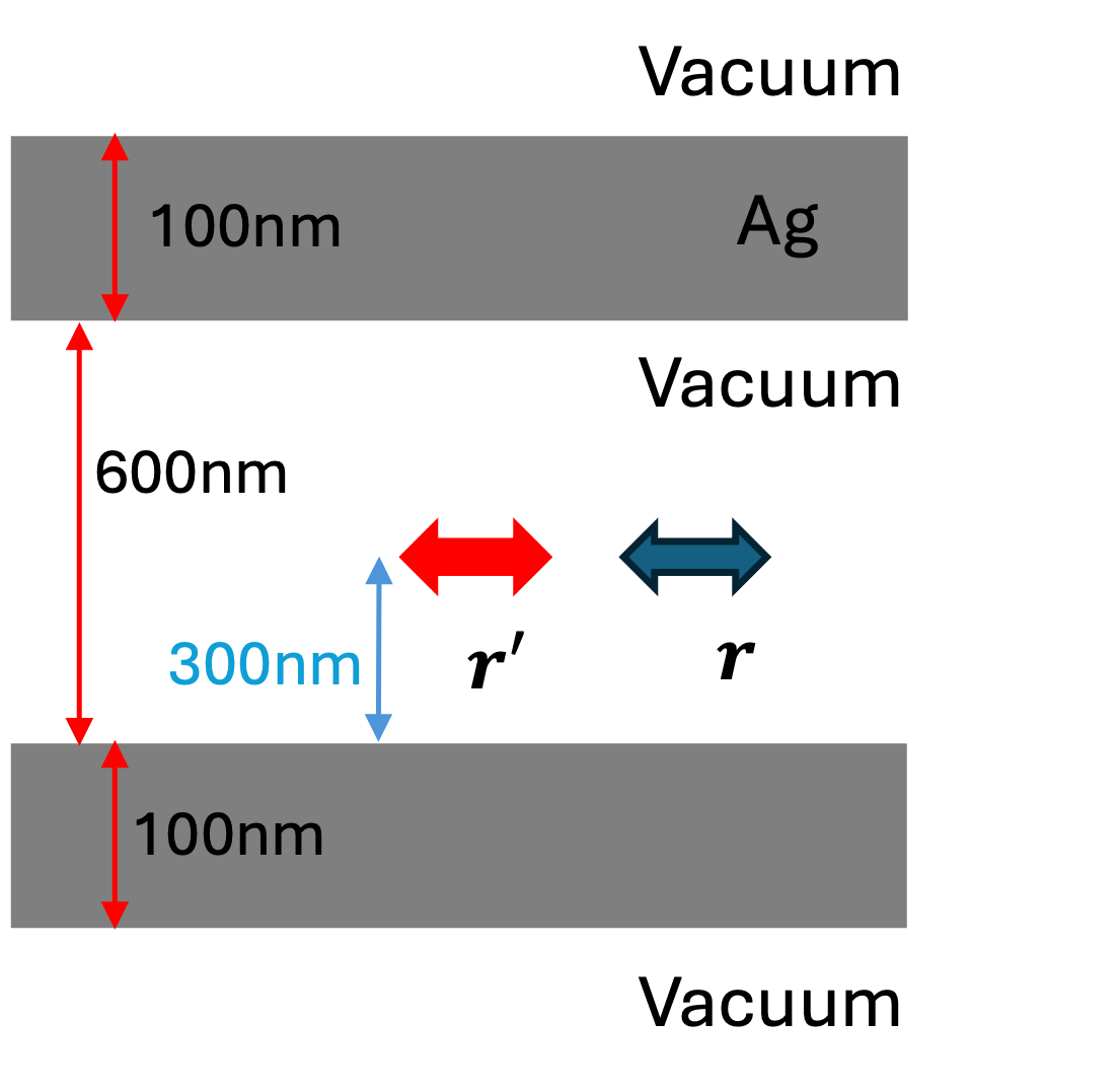
Metal-spacer-metal five-layer stack with the donor and acceptor positioned in the middle of the spacer layer.

Energy grid and segmented sweeps

The example uses a nonuniform segmented energy grid:

simulation:
  spectral_param: energy_eV
  energy_eV:
    segments:
      - min: 0.1
        max: 2.0
        points: 19
      - min: 2.01
        max: 6.0
        points: 400

Use segmented grids when broad spectra need fine resolution only near a plasmonic or guided-mode feature. The same segments format is also accepted by the Mie tutorial.

Integration method

The default example keeps:

simulation:
  integration:
    method: direct

direct is the simplest real-axis quadrature baseline. For validation of plasmonic stacks, compare it against the more robust singularity-aware path:

mqed_GF_NLayer \
  --config-name GF_NLayer_five_layer \
  simulation.integration.method=singularity_aware

Accelerated methods such as hybrid_dcim and pole_aware_hybrid_dcim are available, but should be treated as benchmarked approximations for a specific stack and frequency window rather than automatic replacements for direct quadrature.

Output schema

The N-layer driver writes the shared separation HDF5 layout used by the two-layer Sommerfeld workflow:

green_function_total[M, K, 3, 3]
green_function_vacuum[M, K, 3, 3]
energy_eV[M]
Rx_nm[K]
gf_layout = "separation"

Set output.save_polarization_components: true to add:

green_function_structure[M, K, 3, 3]
green_function_scattering_te[M, K, 3, 3]
green_function_scattering_tm[M, K, 3, 3]

These optional tensors satisfy structure = TE + TM and total = vacuum + structure. TE and TM are scattering-only channels; the analytical homogeneous vacuum tensor is not assigned a TE/TM decomposition.

Here M is the number of energy points and K is the number of lateral separations. This layout can be passed directly to Spectral Density J(\omega), field-enhancement calculations, or quantum dynamics workflows that assume translational symmetry.

Compute spectral density from the N-layer result

Once the Green-function file exists, point the spectral-density config to it:

mqed_calc_spec_dens \
  --config-name spectral_density \
  input_file=/path/to/NLayer_GF_five_layer_Ag_spacer_Emin_0.10_Emax_6.00_419pts_Rx_120nm_3pts.hdf5 \
  output_prefix=spec_dens_nlayer

Curated reference Green-function and spectral-density files are bundled under data/example/GF_data and data/example/spec_dens_data. In those file names, sg_aware means the singularity-aware quadrature result, and pole_hybrid means the pole-aware hybrid DCIM result.

Then plot it with:

mqed_plot_spec_dens \
  --config-name plt_spec_dens_direct_sg \
  input_file=/path/to/spec_dens_1D_1D_Emin_0.10_Emax_6.00_419pts_height_300nm.hdf5

This plots the direct-quadrature spectral-density file. For separation-layout files, choose curves by plot_settings.separation_indices or by physical distances with plot_settings.separation_values_nm.

To compare multiple integration methods, run the spectral-density calculation for each method and then plot them together with one of the comparison configs. The example config configs/plots/plt_spec_dens_direct_sg.yaml selects curves from the direct and singularity-aware files and overlays them.

mqed_plot_spec_dens \
  --config-name plt_spec_dens_direct_sg

This comparison should look like the figure below; it follows the same physical setup as Ref. [Chuang2022spec] and uses the bundled 0, 12, and 120 nm separation curves.

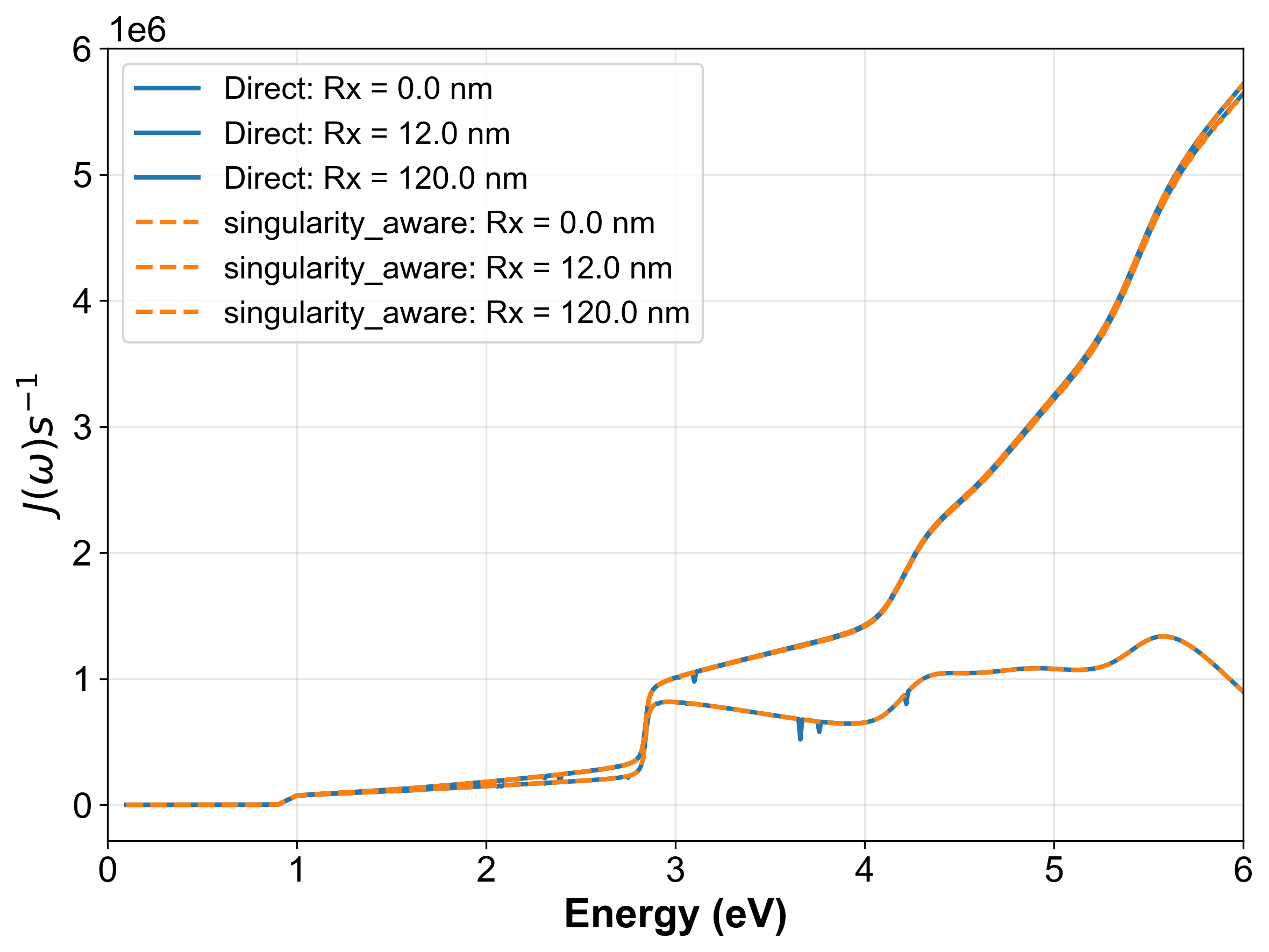
Spectral density for the five-layer cavity from direct and singularity-aware quadrature. The singularity-aware method captures the plasmonic feature more accurately.

The second comparison config overlays the singularity-aware and pole-aware hybrid DCIM results:

mqed_plot_spec_dens \
  --config-name plt_spec_dens_sg_pole_hybrid

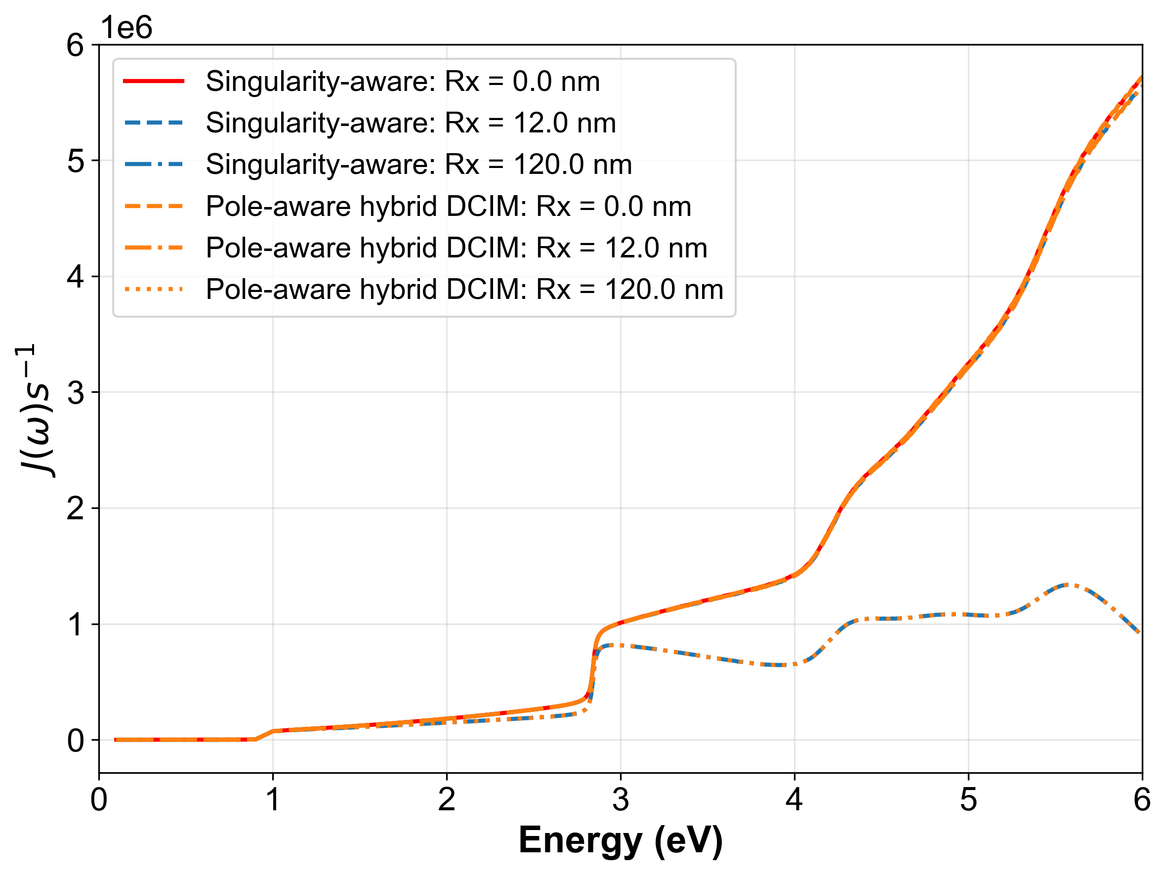
Spectral density for the five-layer cavity from singularity-aware and pole-aware hybrid DCIM methods. The pole-aware hybrid DCIM method provides a good balance between accuracy and computational efficiency.

HPC launcher

For many-frequency sweeps, use the bundled SGE/MPI launcher:

qsub mqed/Dyadic_GF/gf_nlayer_single_job.sh

To run a personal config:

qsub -v GF_CONFIG_NAME=GF_NLayer_my_stack \
     mqed/Dyadic_GF/gf_nlayer_single_job.sh

The script launches mqed_GF_NLayer under mpirun and sets parallel.backend=mpi with parallel.mpi_auto_launch=false so Hydra does not start MPI a second time.

Common mistakes

• Wrong layer index: source_layer is zero-based and must point to the layer containing zD_nm and zA_nm. Internal source layers must be finite. The semi-infinite top exterior is also supported; there zD_nm and zA_nm are non-negative heights above the top-stack interface.

• Expecting arbitrary emitter positions: N-layer output is indexed by lateral separation Rx. Use Mie pair or BEM reconstruction for fully arbitrary 3D emitter positions.

• Trusting accelerated integration without comparison: first validate a candidate method against direct or singularity_aware on a smaller grid.

Next steps

• Spectral Density J(\omega) for converting the N-layer HDF5 file into \(J(\omega)\).

• Mie Green’s Function for Spherical Cavities if your geometry is a spherical cavity or sphere.

• Dyadic Green’s Function via Sommerfeld Integrals for the two-layer baseline workflow.

References

[Chuang2022spec]

Chuang et al., “Chuang, Y.T., Lee, M.W. and Hsu, L.Y., 2022. Tavis-Cummings model revisited: A perspective from macroscopic quantum electrodynamics. Frontiers in Physics, 10, p.980167.”