BEM Vacuum Calibration for Dipoles

Goal

This tutorial shows how to calibrate BEM electric-field amplitudes in vacuum using MQED-QD. You will:

• run a vacuum dipole simulation in MNPBEM,

• compute the complex scaling factor \(p_\mathrm{eff}(\omega)\) with mqed_BEM_compute_peff,

• produce a CSV calibration file used later in Reconstruct Dyadic Green’s Function from BEM.

For implementation details and benchmark context, see the MNPBEM toolbox paper [Hohenester2012BEMVac] and the MQED-QD paper [Liu2026BEMVac].

The calibration relies on matching BEM fields to the analytical vacuum reference:

\[\mathbf{E}_{0}(\mathbf{r}, \omega) = \frac{\omega^2}{\varepsilon_0 c^2} \overline{\overline{\mathbf{G}}}_0(\mathbf{r},\mathbf{r}_0,\omega) \cdot \mathbf{p}.\]

See also

Two-Layer Planar Geometry for dyadic Green’s function definitions and notation.

Prerequisites

• MQED-QD installed (see Installation).

• MATLAB with MNPBEM installed and added to MATLAB path.

• Familiarity with the example script mqed/BEM/MATLAB_script/planar/dipole_vacuum_GF.m.

Step 1: Run the vacuum BEM script

Open mqed/BEM/MATLAB_script/planar/dipole_vacuum_GF.m and set your MNPBEM path:

addpath(genpath('MNPBEMDIR'));

Typical parameters in the script are:

r0 = [0, 0, 2];           % dipole position (nm)
pdir = [0, 0, 1];         % dipole orientation
x_target_min = 5;
x_target_max = 100;
z_target_val = r0(3) + 1; % offset to avoid symmetry-zero lines
enei = 665;               % wavelength (nm)

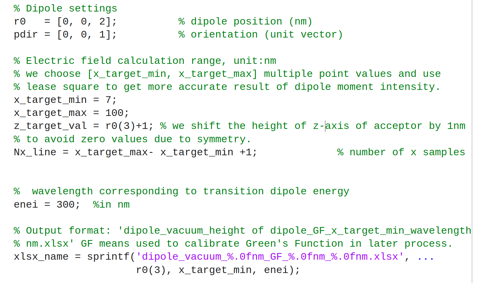
Example MATLAB setup for vacuum dipole calibration: dipole geometry, sampling window, and wavelength settings.

The script writes an Excel file (for example, dipole_vacuum_2nm_GF_5nm_665nm.xlsx) containing the sampled electric field.

Tip

In practice, larger x_target_min (for example 40–50 nm) can improve robustness of the least-squares calibration by reducing near-field oscillatory numerical noise.

Step 2: Compute \(p_\mathrm{eff}\) with MQED-QD

From the repository root:

mqed_BEM_compute_peff

This command uses configs/BEM/compute_peff.yaml by default.

Use a custom config in the same directory:

mqed_BEM_compute_peff --config-name=my_compute_peff

Or load one from any directory:

mqed_BEM_compute_peff --config-dir=/path/to/my/configs --config-name=my_compute_peff

You can combine either approach with direct Hydra overrides:

mqed_BEM_compute_peff --config-name=my_compute_peff sim.lambdas_nm=665

Configuration reference

Key fields in configs/BEM/compute_peff.yaml:

io:
  xlsx_path: ${io.data_dir}/BEM_GF_sample/${sim.lambdas_nm}nm/dipole_vacuum_2nm_GF_${sim.Rx_min_nm}nm_${sim.lambdas_nm}nm.xlsx
  sheet: FieldLine
  output_csv: peff_vs_lambda_${sim.lambdas_nm}nm_${sim.Rx_min_nm}nm.csv

sim:
  Rx_min_nm: 7
  lambdas_nm: 1000
  y_nm: 0.0
  zD_nm: 2.0
  zA_nm: 3.0
  pdir: [0.0, 0.0, 1.0]

dipole:
  p_test_Cm: 1.0

fit:
  drop_small_E0: true
  drop_threshold_rel: 1.0e-12

Expected output

The run writes:

• a Hydra log in outputs/compute_peff/.../compute_peff.log,

• a CSV file such as peff_vs_lambda_665nm_40nm.csv with fitted calibration values.

Example output CSV with fitted calibration quantities (\(p_\mathrm{eff}\) and \(s\)).

This CSV is the direct input for BEM Green’s-function reconstruction in Reconstruct Dyadic Green’s Function from BEM.

References

[Hohenester2012BEMVac]

U. Hohenester and A. Trugler, “MNPBEM - A Matlab toolbox for the simulation of plasmonic nanoparticles,” Computer Physics Communications 183 (2012) 370-381.

[Liu2026BEMVac]

G. Liu, S. Wang, and H. T. Chen, “MQED-QD: An Open-Source Package for Quantum Dynamics Simulation in Complex Dielectric Environments,” arXiv:2603.05378.