Studying quantum emitters above a nanorod using BEM
Goal
This tutorial walks you through simulating the interaction of a quantum emitter with a metallic nanorod using the Boundary Element Method (BEM).
Tip
What is BEM? The Boundary Element Method is a numerical technique that solves Maxwell’s equations only on the surface of a nanostructure, rather than throughout its entire volume. This makes it much more efficient for compact objects like nanorods, nanospheres, and other metallic nanoparticles. Unlike analytical methods, BEM can handle essentially any geometry – you just need a surface mesh.
You will learn how to:
Set up the geometry of a nanorod and a quantum emitter in MNPBEM (a MATLAB toolbox for BEM simulations).
Run BEM simulations to compute the electric field at the emitter position.
Test the convergence of BEM results with respect to mesh refinement (this is essential – without it you cannot trust your results).
Reconstruct the dyadic Green’s function from the BEM output.
By the end you will know how to:
generate BEM field data for an emitter above a nanorod, and
verify that the results are converged before using them in downstream quantum-dynamics simulations.
Note
No MATLAB experience needed. Each code block below is annotated line-by-line so you can follow along even if MATLAB is new to you. You do not need to write MATLAB code from scratch – the scripts are provided and you only need to adjust a few parameters.
Prerequisites
Before starting this tutorial, make sure you have:
Completed BEM Vacuum Calibration for Dipoles and produced the
peffCSV data. (This calibrates the BEM solver against an analytically known case.)MATLAB with the MNPBEM toolbox installed. MNPBEM is used to generate the geometry-specific BEM field files.
MQED-QD installed (see Installation).
Tip
If you are unsure whether MNPBEM is installed correctly, open MATLAB and
type help trirod. You should see the documentation for the trirod
function. If not, check that the MNPBEM folder is on your MATLAB path.
Step 1: Visualise the nanorod geometry (optional)
Before running any simulation it is helpful to visualise the nanorod and the
emitter position so you can confirm everything is set up correctly.
Open the MATLAB script nanorod/illustration_nanorod.m.
The first section defines the nanorod dimensions and mesh resolution. You can think of this as building a 3-D wireframe model of the nanorod:
% --- Nanorod geometry ---
diameter = 20;   % diameter in nm
height   = 200;  % length in nm

n = [30, 15, 100];  % discretisation points [nphi, ntheta, nz]

pmesh = trirod(diameter, height, n, 'triangles');

% Rotate so the long axis lies along x
pmesh = rot(pmesh, -90, [0 1 0]);
diameterandheightset the physical size of the nanorod (in nm). Change these to match the nanorod you want to simulate.ncontrols how finely the surface is meshed. Each number corresponds to a direction:nphi(around the circumference),ntheta(end caps), andnz(along the length). Larger values give a smoother surface but take longer to compute.trirodcreates the triangulated surface mesh;rotrotates it so that the long axis points along x (horizontal).
Next, we shift the nanorod so that its left edge sits at x = 0 and its top
surface sits at z = 0. This is a bookkeeping step that makes it easier to
place emitters at known heights above the surface:
x_left = min(pmesh.pos(:,1));
z_top  = max(pmesh.pos(:,3));
pmesh  = shift(pmesh, [-x_left, 0, -z_top]);
Now we create the comparticle object. This tells MNPBEM about the
dielectric environment – which regions are metal and which are vacuum. We
then place a z-oriented dipole (representing our quantum emitter) 2 nm
above the centre of the nanorod:
% Particle: outside medium = 1 (vacuum), inside metal = 2 (silver)
p = comparticle(epstab, {pmesh}, [2,1], 1, op);

% Dipole position: centre of the rod, 2 nm above the surface
x_middle = 0.5 * (max(pmesh.pos(:,1)) + min(pmesh.pos(:,1)));
z_top    = max(pmesh.pos(:,3));
r0   = [x_middle, 0, z_top + 2];   % [x, y, z] in nm
pdir = [0, 0, 1];                   % z-polarised dipole

pt1 = compoint(p, r0, op);   % register emitter location
dip = dipole(pt1, pdir, op); % create dipole source
Finally, we plot the mesh together with the dipole position:
figure('Units','pixels','Position',[100 100 1200 900]);
hold on; axis equal;

% Nanorod surface
plot(pmesh, 'FaceColor',[0.8 0.8 0.85], ...
            'EdgeColor',[0.2 0.2 0.2]);

% Dipole marker
plot3(r0(1), r0(2), r0(3), 'ro', ...
      'MarkerFaceColor','r', 'MarkerSize',8);

xlabel('x (nm)'); ylabel('y (nm)'); zlabel('z (nm)');
view(35, 20); grid off;
title('Nanorod mesh + dipole position');
You should see something like the figure below. The red dot marks the dipole (emitter) position:
Step 2: Test convergence with respect to mesh refinement
In BEM the accuracy of the result depends on how finely the surface is discretised. Before trusting any simulation you should verify that the quantities of interest have converged – that is, they stop changing significantly when you make the mesh finer.
Tip
Why convergence matters. A coarse mesh is fast to compute but may give inaccurate results. A very fine mesh gives accurate results but takes much longer. The convergence test tells you the “sweet spot” – the coarsest mesh that is still accurate enough.
Open the MATLAB script nanorod/test_convergence_nanorod.m.
We use a 1000 nm long, 20 nm diameter silver nanorod as an example. The dipole wavelength is 665 nm and the dipole is z-polarised:
diameter = 20;     % nm
height   = 1000;   % nm

enei = 665;        % dipole wavelength in nm
pdir = [0, 0, 1];  % z-polarised
The key idea is to run the same simulation with increasingly fine meshes and
check when the results stop changing. Each row in n_list specifies
[nphi, ntheta, nz] – the number of discretisation points in each
direction. Notice that we only increase nz (along the rod length) because
that is the most sensitive direction for this geometry:
n_list = {
    [20, 10,  10];
    [20, 10,  30];
    [20, 10,  50];
    [20, 10,  80];
    [20, 10, 120];
    [20, 10, 150];
    [20, 10, 180];
    [20, 10, 210];
    [20, 10, 240];
};
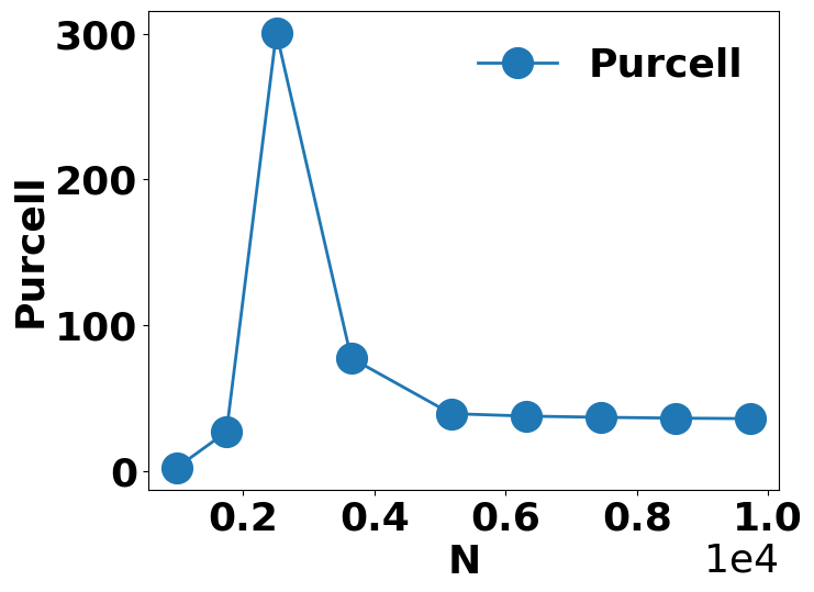
The script loops over each mesh, builds the nanorod, runs a BEM solve, and records two quantities that we will use to judge convergence:
Purcell factor (
F_tot) – measures how much the nanorod enhances the emitter’s decay rate compared to vacuum. A stable Purcell factor means the electromagnetic environment is well-resolved.Electric field at a probe point 3 nm from the dipole (
Ez_probe) – a particularly sensitive check on near-field accuracy because the field changes rapidly close to the surface.
for k = 1:numel(n_list)
    n = n_list{k};
    fprintf('Mesh %d: nphi=%d, ntheta=%d, nz=%d\n', k, n);

    % --- Build mesh and shift to standard position ---
    rodmesh = trirod(diameter, height, n, 'triangles');
    rodmesh = rot(rodmesh, -90, [0 1 0]);

    x_left_before = min(rodmesh.pos(:,1));
    z_top_before  = max(rodmesh.pos(:,3));
    rodmesh = shift(rodmesh, [-x_left_before, 0, -z_top_before]);

    x_middle = round(0.5 * (min(rodmesh.pos(:,1)) ...
                           + max(rodmesh.pos(:,1))));
    z_top    = max(rodmesh.pos(:,3));

    p = comparticle(epstab, {rodmesh}, [2,1], 1, op);
    Nfaces(k) = size(rodmesh.faces, 1);

    % --- Dipole + BEM solve ---
    r0        = [x_middle, 0, 8];           % 8 nm above surface
    pt1       = compoint(p, r0, op);
    probe_pt  = [r0(1)+3, 0, r0(3)];       % 3 nm away from dipole
    dip       = dipole(pt1, pdir, op);
    bem       = bemsolver(p, op);
    sig       = bem \ dip(p, enei);

    % Purcell factor
    [F_tot, F_rad]  = dip.decayrate(sig);
    F_tot_list(k)   = F_tot;

    % Near-field at probe point
    pt_probe = compoint(p, probe_pt, op);
    emesh    = meshfield(p, pt_probe.pos(:,1), ...
                            pt_probe.pos(:,2), ...
                            pt_probe.pos(:,3), op);
    e_probe     = emesh(sig) + emesh(dip.field(emesh.pt, enei));
    Ez_probe(k) = e_probe(3);
end
After the loop the script saves the convergence data to a CSV file so you can inspect the numbers later. This is useful for record-keeping and for deciding which mesh to use in Step 3:
convTable = table(Nfaces(:), F_tot_list(:), ...
                  real(Ez_probe(:)), imag(Ez_probe(:)), ...
    'VariableNames', {'Nelem','Purcell','ReEz','ImEz'});

csvFile = fullfile('convergence_data', ...
    sprintf('conv_h%gnm_pos%gnm_D%gnm_dip%.0fnm.csv', ...
            r0(3), r0(1), diameter, enei));
writetable(convTable, csvFile);
The script also produces publication-quality convergence plots. If you prefer
Python over MATLAB for plotting, a ready-made alternative is provided in
nanorod/plot_convergence.py.
You should see the Purcell factor and the real/imaginary parts of the near-field plateau (flatten out) as the mesh is refined. When the curves become flat, the results are converged:
Note
Convergence behaviour depends on the geometry, the wavelength, and the dipole position. Always run a convergence test for your specific setup before using the results in production simulations. If you change any of these parameters, you should re-run the convergence check.
Step 3: Generate BEM field data and reconstruct the Green’s function
Once you have identified a converged mesh (from Step 2), you are ready to generate the full BEM field data needed to reconstruct the dyadic Green’s function. This is the main computational step of the tutorial.
Open the MATLAB script nanorod/dipole_silver_nanorod_GF.m. Most of the
geometry setup is identical to what you saw in Steps 1 and 2; the new part is
that we compute the electric field over a line of target positions – one for
each acceptor emitter you want to study.
Define the target positions and output file:
% Range of target positions along x (in nm)
x_target_min = r0(1) + 1;
N_num        = 30;              % number of acceptor emitters
x_target_max = r0(1) + 8*N_num;
z_target_val = r0(3);           % same height as the dipole

Nx_line = (x_target_max - x_target_min) + 1;  % number of x samples
enei    = 665;                  % wavelength in nm

xlsx_name = sprintf( ...
    'dipole_silver_nanorod_GF_%.0fnm_pos_%.0f_height_%.0fnm_D_%.0fnm_%.0f.xlsx', ...
    enei, r0(1), r0(3), diameter, test_number);
N_num– the number of acceptor emitters you want to study (here 30). Increase this if you need more emitters in your quantum-dynamics simulation.x_target_min/x_target_max– the x-range over which the electric field is computed. Each point corresponds to a potential acceptor position.z_target_val– the height of the acceptors above the nanorod surface, set equal to the donor height (so all emitters are in the same plane).
Loop over three orthogonal dipole orientations:
To reconstruct the full 3 x 3 dyadic Green’s function we need the electric field response to dipoles polarised along all three Cartesian directions (x, y, and z). The script loops over them automatically:
for j = 1:3
    dip = dipole(pt1, pdirs(j,:), op);
    sig = bem \ dip(p, enei);

    [tot, ~] = dip.decayrate(sig);
    Ftot(j)  = tot;

    % Total field = scattered + direct
    e     = emesh(sig) + emesh(dip.field(emesh.pt, enei));
    Eline = squeeze(e);   % N x 3

    G(:,1,j) = pref * Eline(:,1);
    G(:,2,j) = pref * Eline(:,2);
    G(:,3,j) = pref * Eline(:,3);
end
Save to xlsx:
The nine Green’s function components (each with real and imaginary parts) are
written to an Excel sheet named DyadicG. The self-interaction Purcell
factors for each dipole orientation go to a sheet named G_self:
writetable(T,     xlsx_name, 'Sheet', 'DyadicG');
writetable(Tself, xlsx_name, 'Sheet', 'G_self');
Warning
The Green’s function elements in the xlsx file are not in SI units. You must apply the prefactor obtained from BEM Vacuum Calibration for Dipoles to convert them before using them in MQED-QD. Forgetting this step is a common source of incorrect results.
Also make sure to record all simulation parameters (wavelength, dipole position, nanorod dimensions) so that results can be reproduced later.
Reconstruct the Green’s function in MQED-QD:
Following Reconstruct Dyadic Green’s Function from BEM, run mqed_BEM_reconstruct_GF
with a configuration like the one below. You mainly need to update the file
paths and parameters to match your simulation:
parameters:
  energy_eV: 1.864
  lambda_nm: 665
  zD_nm: 8
  zA_nm: 8
  geometry: "nanorod"
  material: "Ag"
  dipole_position_nm: 500

io:
  xlsx_path: ${oc.env:MQED_ROOT,${hydra:runtime.cwd}}/mqed/data/example/BEM_data/dipole_silver_nanorod_GF_665nm_pos_500_height_8nm_D_20nm_1.xlsx
  peff_path: ${oc.env:MQED_ROOT,${hydra:runtime.cwd}}/mqed/data/example/BEM_data/peff_vs_lambda_665nm_50nm.csv
  output_file: BEM_GF_${parameters.geometry}_${parameters.material}_${parameters.lambda_nm}nm_height_${parameters.zD_nm}nm_pos_${parameters.dipole_position_nm}nm.hdf5
In practice you usually only need to change three things:
io.xlsx_path– point this to the BEM field xlsx file from this step.io.peff_path– point this to the vacuum calibration CSV from BEM Vacuum Calibration for Dipoles.The
parametersentries – update geometry, material, wavelength, and height to match your simulation.
Tip
The ${oc.env:MQED_ROOT,...} syntax is Hydra’s way of looking up the
project root directory. You generally do not need to change it unless you
have installed MQED-QD in an unusual location.
Expected output
If everything went well, the reconstruction command writes:
a Hydra log under
outputs/reconstruct_GF/.../reconstruct_GF.log(check this first if anything looks wrong),an HDF5 file containing the dyadic Green’s function (the filename is set by
io.output_filein the config).
You can then feed this HDF5 file into downstream quantum-dynamics simulations – for example:
run
mqed_nhseto study non-Hermitian skin effect dynamics (see Quantum Dynamics), oranalyse MSD and participation ratio (see Plotting & Analysis).
Warning
This tutorial uses xlsx format for the BEM field output because we assume (and verify) translational symmetry along the nanorod axis. This means the Green’s function only depends on the separation between donor and acceptor, not their absolute positions.
For more complex geometries without such symmetry you would need to
construct a four-dimensional array of shape (N, N, 3, 3) and store it
in HDF5 for efficiency. See the API reference for save_hdf5 for
details.
Troubleshooting
- MATLAB runs out of memory during the convergence test.
Fine meshes can be memory-intensive. Try reducing
nphiandnthetafirst, and increasenzin smaller increments. Close other MATLAB variables withclearbefore running the solve.- The Purcell factor does not converge.
Make sure the dipole is far enough from the surface (at least 2 nm). Dipoles very close to the metal surface require extremely fine meshes. Also verify that the dielectric function (
epstab) is set correctly.- The xlsx file is empty or has unexpected values.
Check that the emitter wavelength (
enei) matches the plasmon resonance of your nanorod. Far from resonance the fields are very small and may appear to be zero.- Hydra complains about missing config keys.
Double-check that the YAML indentation is correct (use spaces, not tabs) and that all required fields are present. See Installation for config file locations.
See also
Field Enhancement – compute the field enhancement using the Green’s function produced here.
Quantum Dynamics – run Lindblad or NHSE dynamics with this Green’s function as input.