Field Enhancement
Goal
In this tutorial you will compute the electric field enhancement — the dipole-dipole interaction (DDI) ratio \(V_{\alpha\beta}/V_{0,\alpha\beta}\) and the generalised dissipation ratio \(\Gamma_{\alpha\beta}/\Gamma_{0,\alpha\beta}\) — from a previously cached dyadic Green’s function.
By the end you will know how to:
run the
mqed_FEcommand with default and custom parameters,choose donor and acceptor orientations,
select which components (real, imaginary, or both) to plot,
locate and interpret the output figure.
See also
Macroscopic QED Framework for the relation between the electric field enhancement and the dyadic Green’s function.
Prerequisites
Make sure you have installed the package and activated the environment as described in Installation.
This tutorial uses example data bundled under data/example/GF_data/.
To generate your own Green’s function cache, see
Dyadic Green’s Function via Sommerfeld Integrals.
Quick start
Run from the repository root with all defaults:
mqed_FE
This uses the YAML configuration at configs/analysis/FE.yaml.
The default settings compute the enhancement from the bundled example file
data/example/GF_data/Fresnel_GF_planar_Ag_height_8nm_665nm.hdf5 with
donor and acceptor oriented at the magic angle in the XY plane.
Both \(V_{\alpha\beta}/V_{0,\alpha\beta}\) (real) and
\(\Gamma_{\alpha\beta}/\Gamma_{0,\alpha\beta}\) (imag) are
plotted by default.
Tip
The example data ships with the repository under data/example/.
No prior simulation run is required to follow this tutorial.
Customising the run
Override individual parameters on the command line using Hydra syntax:
mqed_FE orientations.donor.phi_deg=0.0 orientations.acceptor.phi_deg=0.0
Use a different YAML in the same config directory
(configs/analysis/):
mqed_FE --config-name=my_FE
Use a YAML from an arbitrary directory:
mqed_FE --config-dir=/path/to/my/configs --config-name=my_FE
Tip
You can combine --config-name (or --config-dir) with individual
parameter overrides:
mqed_FE --config-name=my_FE plot_settings.dpi=300
Configuration reference
The full default configuration file
(configs/analysis/FE.yaml) is reproduced below with
annotations.
# ── Input ───────────────────────────────────────────────
input_file: ${oc.env:MQED_ROOT,${hydra:runtime.cwd}}/data/example/GF_data/Fresnel_GF_planar_Ag_height_8nm_665nm.hdf5

# ── Orientations ────────────────────────────────────────
orientations:
  donor:    { theta_deg: 90.0, phi_deg: "magic" }
  acceptor: { theta_deg: 90.0, phi_deg: "magic" }

# ── Plot settings ───────────────────────────────────────
plot_settings:
  save_plot: true
  dpi: 400

  # choose x-range by value or by indices, not both
  x_range_nm: [0.0, 100.0]       # mask points where 0 ≤ Rx_nm ≤ 100
  # x_index_range: [0, 9]        # alternative: mask first 10 points

  components: ["real", "imag"]    # options: ["real"], ["imag"], ["real","imag"]

  # Text & style
  xlabel: "Donor–Acceptor Distance (nm)"
  ylabel: "Enhancement"
  title_template: "Emitter energy = {energy:.3f} eV"
  legend:
    real_label: "$V_{\\alpha\\beta}/ V_{0,\\alpha\\beta}$"
    imag_label: "$\\Gamma_{\\alpha\\beta}/ \\Gamma_{0,\\alpha\\beta}$"

  lw: 1
  real_style: "r--"
  imag_style: "b--"

  xscale: linear                  # or "log"
  yscale: linear                  # or "log"

  # Optional axis limits
  xlim: [0, 50]                   # e.g., [0, 500]
  ylim: null                      # e.g., [0, 10]
  filename_prefix: "enhancement_magic_angle"
  grid: true
Parameter |
Description |
Default |
|---|---|---|
|
Path to the cached dyadic Green’s function HDF5 file. |
|
|
Polar and azimuthal angles of the donor dipole. |
|
|
Polar and azimuthal angles of the acceptor dipole. |
|
|
Which ratios to plot: |
|
|
Horizontal distance window for the plot (nm). |
|
|
Matplotlib axis limits for the x-axis. |
|
Expected output
After the simulation finishes, a success message is printed to the terminal
(and to the Hydra log file
outputs/FE/.../FE.log):
2025-10-24 11:40:02.818 | SUCCESS | mqed.analysis.FE:plot_field_enhancement:149
- Simulation complete. Output saved to:
  /.../MacroscopicQED/outputs/FE/Y-M-D/H-M-S/enhancement_magic_angle_1.864eV.png
The output is a PNG figure showing the selected enhancement components as a function of donor-acceptor distance.
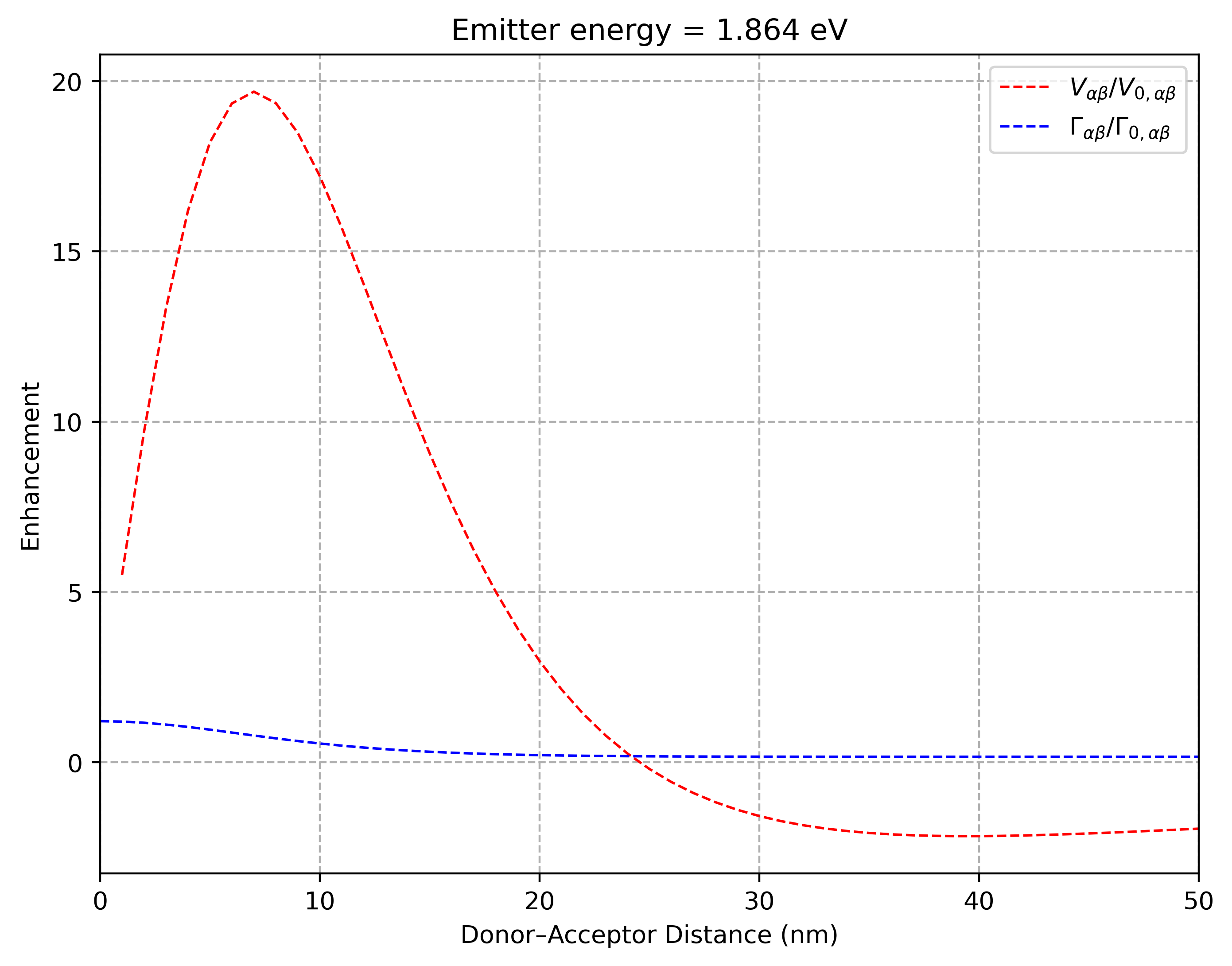
Field enhancement vs donor-acceptor distance.
Resonance Energy Transfer (mqed_RET)
The mqed_FE command above plots the coherent and incoherent channels
(\(V_{\alpha\beta}/V_{0,\alpha\beta}\) and
\(\Gamma_{\alpha\beta}/\Gamma_{0,\alpha\beta}\)) separately.
A companion command, mqed_RET, computes the resonance energy transfer
enhancement factor \(\gamma\) — a single scalar that captures the
overall RET enhancement by the dielectric environment:
See Resonance Energy Transfer Enhancement Factor for the theoretical background.
Quick start
mqed_RET
This uses the configuration at configs/analysis/RET.yaml, which is
structured identically to the FE.yaml used above. The same input HDF5
file, orientation parameters, and Hydra override syntax all apply:
# Override dipole orientations
mqed_RET orientations.donor.phi_deg=0.0 orientations.acceptor.phi_deg=0.0

# Use a custom config
mqed_RET --config-name=my_RET
The output is a plot of \(\gamma\) versus donor–acceptor distance. While
mqed_FE separates the real and imaginary parts to reveal the individual
coherent and incoherent channels, mqed_RET shows their combined effect as
a single enhancement factor — useful for a quick assessment of whether a given
dielectric structure enhances or suppresses resonance energy transfer overall.
What’s next?
Quantum Dynamics — use the Green’s function and field enhancement results to drive open quantum dynamics.
Plotting & Analysis — visualise the enhancement spectra and other transport observables.