Two-Layer Planar Geometry

This section derives the scattering dyadic Green’s function for a planar two-layer geometry — the simplest nontrivial system in which a dielectric interface modifies the electromagnetic field. We state the Fresnel reflection coefficients for s- and p-polarised waves, then give the resulting scattering Green’s function as Sommerfeld integrals in cylindrical coordinates. The mathematical discussion follows [Wu2018]; a full step-by-step derivation (boundary conditions, coordinate rotation, Bessel-function identities) can be found in [Novotny2012] Ch. 10 and [Sarabandi]. A detailed derivation is also included in this PDF.

Geometry

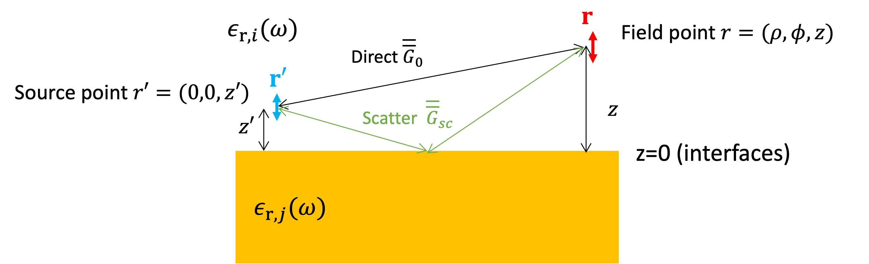
Two-layer planar geometry. The source (donor) is in medium i above the interface and the field point (acceptor) is at lateral separation \(\rho\).

The source (donor) is at \(\mathbf{r}' = (0, 0, z')\) in medium i (above the interface) and the field point (acceptor) is at \(\mathbf{r} = (\rho, \varphi, z)\), also in medium i. The interface sits at \(z = 0\).

Fresnel Reflection Coefficients

Applying the electromagnetic boundary conditions (tangential \(\mathbf{E}\) and \(\mathbf{H}\) continuous across the interface) to s- and p-polarised plane waves yields the Fresnel reflection coefficients.

Define the perpendicular wave vector in medium \(l\):

(1)\[K_{z,l}(\omega, k_\rho) = \sqrt{\varepsilon_{r,l}(\omega)\,\frac{\omega^2}{c^2} - k_\rho^2}, \qquad l = i, j,\]

where \(k_\rho\) is the in-plane wave vector magnitude and the branch is chosen so that \(\mathrm{Im}\,K_{z,l} \geq 0\) (outgoing/evanescent waves).

s-polarisation (TE — electric field parallel to the interface):

(2)\[R_s(k_\rho, \omega) = \frac{K_{z,i} - K_{z,j}}{K_{z,i} + K_{z,j}}.\]

p-polarisation (TM — magnetic field parallel to the interface):

(3)\[R_p(k_\rho, \omega) = \frac{\varepsilon_{r,j}\,K_{z,i} - \varepsilon_{r,i}\,K_{z,j}} {\varepsilon_{r,j}\,K_{z,i} + \varepsilon_{r,i}\,K_{z,j}}.\]

Scattering Green’s Function

The total dyadic Green’s function decomposes as

\[\overline{\overline{\mathbf{G}}}(\mathbf{r}, \mathbf{r}', \omega) = \overline{\overline{\mathbf{G}}}_0(\mathbf{r}, \mathbf{r}', \omega) + \overline{\overline{\mathbf{G}}}_\mathrm{Sc}(\mathbf{r}, \mathbf{r}', \omega),\]

where \(\overline{\overline{\mathbf{G}}}_0\) is the closed-form vacuum Green’s function and \(\overline{\overline{\mathbf{G}}}_\mathrm{Sc}\) encodes the effect of the interface.

Vacuum Green’s Function

The free-space dyadic Green’s function has the closed-form analytical expression

\[\overline{\overline{\mathbf{G}}}_0(\mathbf{r}_\alpha,\mathbf{r}_\beta,\omega) = \frac{e^{ik_0 R_{\alpha\beta}}}{4\pi R_{\alpha\beta}} \Big[ \left(\overline{\overline{\mathbf{I}}}_3 - \mathbf{e}_\mathrm{R}\mathbf{e}_\mathrm{R}\right) + \left(3\mathbf{e}_\mathrm{R}\mathbf{e}_\mathrm{R} - \overline{\overline{\mathbf{I}}}_3\right) \left(\frac{1}{(k_0 R_{\alpha\beta})^{2}} - \frac{i}{k_0 R_{\alpha\beta}}\right) \Big],\]

where \(R_{\alpha\beta} = |\mathbf{r}_\alpha - \mathbf{r}_\beta|\) is the distance between the source and field points, \(\mathbf{e}_\mathrm{R} = (\mathbf{r}_\alpha - \mathbf{r}_\beta)/R_{\alpha\beta}\) is the unit vector along that direction, \(\overline{\overline{\mathbf{I}}}_3\) is the \(3\times 3\) identity tensor, and \(k_0 = \omega/c\) is the free-space wave number.

Scattering Part

In cylindrical coordinates the scattering part is given by the Sommerfeld integral:

\[\overline{\overline{\mathbf{G}}}_\mathrm{Sc}(\rho, \varphi, z, z', \omega) = \int_{0}^{+\infty} \frac{i\,dk_{\rho}}{4\pi} \Big[ R_s\,\overline{\overline{\mathbf{M}}}^{(s)} + R_p\,\overline{\overline{\mathbf{M}}}^{(p)} \Big]\, e^{iK_{z,i}(k_{\rho},\,\omega)(z+z')}.\]

\(\mathbf{M}^{(s)}\) — s-wave contribution

(4)\[\begin{split}\overline{\overline{\mathbf{M}}}^{(s)}(k_{\rho}, \omega) = \frac{k_{\rho}}{2\,K_{z,i}} \begin{pmatrix} J_0 + \cos 2\varphi\;J_2 & \sin 2\varphi\;J_2 & 0 \\ \sin 2\varphi\;J_2 & J_0 - \cos 2\varphi\;J_2 & 0 \\ 0 & 0 & 0 \end{pmatrix},\end{split}\]

where \(J_n = J_n(k_\rho \rho)\) are Bessel functions of the first kind. The s-wave has no \(z\)-component because the electric field lies entirely in the interface plane.

\(\mathbf{M}^{(p)}\) — p-wave contribution

(5)\[\begin{split}\overline{\overline{\mathbf{M}}}^{(p)}(k_{\rho}, \omega) = \frac{-k_{\rho}\,K_{z,i}}{2\,k_i^2} \begin{pmatrix} J_0 - \cos 2\varphi\;J_2 & -\sin 2\varphi\;J_2 & \dfrac{2i\,k_{\rho}}{K_{z,i}}\cos\varphi\;J_1 \\[6pt] -\sin 2\varphi\;J_2 & J_0 + \cos 2\varphi\;J_2 & \dfrac{2i\,k_{\rho}}{K_{z,i}}\sin\varphi\;J_1 \\[6pt] -\dfrac{2i\,k_{\rho}}{K_{z,i}}\cos\varphi\;J_1 & -\dfrac{2i\,k_{\rho}}{K_{z,i}}\sin\varphi\;J_1 & -\dfrac{2\,k_{\rho}^2}{K_{z,i}^2}\;J_0 \end{pmatrix}.\end{split}\]

The p-wave carries all the \(z\)-components of the scattered field.

Sommerfeld Integrals (Implementation)

For numerical evaluation, the Fresnel coefficients and common prefactors are absorbed into six Sommerfeld integrals over the in-plane wave vector \(k_\rho\), each involving the phase factor \(e^{i K_{z,i}(z + z')}\):

(6)\[\begin{split}\begin{aligned} I_1 &= \int_0^\infty \frac{R_s\,k_\rho}{2\,K_{z,i}}\; J_0(k_\rho\rho)\;e^{iK_{z,i}(z+z')}\,dk_\rho, \\[4pt] I_2 &= \int_0^\infty \frac{R_s\,k_\rho}{2\,K_{z,i}}\; J_2(k_\rho\rho)\;e^{iK_{z,i}(z+z')}\,dk_\rho, \\[4pt] I_3 &= \int_0^\infty \frac{R_p\,k_\rho\,K_{z,i}}{2\,k_0^2}\; J_0(k_\rho\rho)\;e^{iK_{z,i}(z+z')}\,dk_\rho, \\[4pt] I_4 &= \int_0^\infty \frac{R_p\,k_\rho\,K_{z,i}}{2\,k_0^2}\; J_2(k_\rho\rho)\;e^{iK_{z,i}(z+z')}\,dk_\rho, \\[4pt] I_5 &= \int_0^\infty \frac{i\,R_p\,k_\rho^2}{k_0^2}\; J_1(k_\rho\rho)\;e^{iK_{z,i}(z+z')}\,dk_\rho, \\[4pt] I_6 &= \int_0^\infty \frac{R_p\,k_\rho^3}{K_{z,i}\,k_0^2}\; J_0(k_\rho\rho)\;e^{iK_{z,i}(z+z')}\,dk_\rho, \end{aligned}\end{split}\]

where \(k_0 = \omega/c\). In the implementation (mqed.Dyadic_GF.GF_Sommerfeld) the integration is split at \(k_\rho = k_0\) (the propagating/evanescent boundary) for numerical accuracy and evaluated with scipy.integrate.quad_vec().

Implementation

The class mqed.Dyadic_GF.GF_Sommerfeld.Greens_function_analytical evaluates these integrals for arrays of energies and lateral separations \(\rho\). See the Dyadic Green’s Function via Sommerfeld Integrals tutorial for usage and the Dyadic_GF/ — Green’s Function Computation section for all available configuration parameters.

References

[Wu2018]

J. S. Wu, Y. C. Lin, Y. L. Sheu, and L. Y. Hsu, “Characteristic distance of resonance energy transfer coupled with surface plasmon polaritons,” J. Phys. Chem. Lett. 9, 7032–7039 (2018).

[Novotny2012]

L. Novotny and B. Hecht, Principles of Nano-Optics, 2nd ed. (Cambridge University Press, 2012), Ch. 10.

[Sarabandi]

K. Sarabandi, “Dyadic Green’s function,” Lecture Notes, University of Michigan.