Reconstruct Dyadic Green’s Function from BEM
Goal
This tutorial explains how to reconstruct a dyadic Green’s function from BEM electric-field output using MQED-QD. The reconstruction uses the calibration factor from BEM Vacuum Calibration for Dipoles:
For numerical details and methodology context, see the MNPBEM toolbox paper [Hohenester2012BEMRec] and the MQED-QD package paper [Liu2026BEMRec].
By the end you will know how to:
generate BEM field data for a target geometry,
run
mqed_BEM_reconstruct_GF,optionally compare reconstructed dyadics against Sommerfeld results for planar validation.
Prerequisites
Completed BEM Vacuum Calibration for Dipoles and produced
peffCSV data.MATLAB + MNPBEM setup for generating geometry-specific BEM field files.
MQED-QD installed (see Installation).
Step 1: Generate BEM field data for your geometry
For planar silver, the example MATLAB script is
mqed/BEM/MATLAB_script/planar/dipole_silver_planar_GF.m.
Typical editable parameters include:
r0 = [0, 0, 2];
x_target_min = 1;
x_target_max = 400;
z_target_val = 2;
enei = 1000;
The script writes an Excel file with electric-field samples used by
mqed_BEM_reconstruct_GF.
Warning
The provided planar script includes a virtual nanosphere placeholder from a more general setup. If MATLAB meshing fails, adjust geometric discretization parameters in the script before rerunning.
Step 2: Reconstruct the Green’s function
Run the packaged planar example:
mqed_BEM_reconstruct_GF --config-dir=mqed/BEM/MATLAB_script/planar --config-name=example_reconstruct_GF
Or run with the default project config:
mqed_BEM_reconstruct_GF
Default config path:
configs/BEM/reconstruct_GF.yaml
Example planarly validated config path:
mqed/BEM/MATLAB_script/planar/example_reconstruct_GF.yaml
Configuration reference
Core fields for reconstruction are:
parameters:
  energy_eV: 1.864
  lambda_nm: 665
  zD_nm: 8
  zA_nm: 8
  geometry: "planar"   # e.g. planar, nanorod, sphere
  material: "Ag"
  dipole_position_nm: 500

io:
  xlsx_path: ${oc.env:MQED_ROOT,${hydra:runtime.cwd}}/mqed/BEM/MATLAB_script/planar/dipole_silver_planar_height_8nm_GF_665nm.xlsx
  peff_path: ${oc.env:MQED_ROOT,${hydra:runtime.cwd}}/mqed/BEM/MATLAB_script/planar/peff_vs_lambda_665nm_50nm.csv
  output_file: BEM_GF_${parameters.geometry}_${parameters.material}_${parameters.lambda_nm}nm_height_${parameters.zD_nm}nm_pos_${parameters.dipole_position_nm}nm.hdf5
In practice, you usually only need to update:
io.xlsx_path(BEM field output),io.peff_path(vacuum calibration CSV),geometry/material/wavelength/height entries under
parameters.
Expected output
The command writes:
a Hydra log under
outputs/reconstruct_GF/.../reconstruct_GF.log,an HDF5 dyadic Green’s function file specified by
io.output_file.
Optional validation against Sommerfeld (planar only)
For planar systems, you can compare reconstructed BEM dyadics to Sommerfeld results using:
mqed_BEM_compare_dyadic
Configuration file:
configs/BEM/compare_bem_dyadic.yaml
That command exports a CSV with selected dyadic components from both methods,
which you can post-process using mqed/BEM/verify_bem_fresnel.py.
python -m mqed.BEM.verify_bem_fresnel path/to/csv_file.csv
User needs to update the CSV path in the script before running. The output gives the relative error between BEM and Sommerfeld dyadics:
| INFO     | __main__:main:83 - s_Gxx = 0.726759+0.000000j  (rel. RMS after scaling = 6.826349e-06)
| INFO     | __main__:main:75 - Component Gxy contains only zero values, skipping scale fit.
| INFO     | __main__:main:83 - s_Gxz = 0.726448-0.000008j  (rel. RMS after scaling = 2.133498e-03)
| INFO     | __main__:main:75 - Component Gyx contains only zero values, skipping scale fit.
| INFO     | __main__:main:83 - s_Gyy = 0.726758+0.000000j  (rel. RMS after scaling = 3.834833e-06)
| INFO     | __main__:main:83 - s_Gzx = 0.726764-0.000007j  (rel. RMS after scaling = 3.914327e-04)
| INFO     | __main__:main:83 - s_Gzz = 0.726759+0.000000j  (rel. RMS after scaling = 2.192826e-05)
| INFO     | __main__:main:90 - s_avg  = 0.726697-0.000003j  (averaged over 5 components)
| SUCCESS  | __main__:main:101 - Mean rel. RMS error (using s_avg) = 5.636888e-04 over 5 components
Plot the calibration/verification accuracy
After running mqed_BEM_compare_dyadic and mqed.BEM.verify_bem_fresnel,
you can reproduce the calibration-distance accuracy figure used in our workflow:
python -m mqed.BEM.accuracy_plot
This script plots \(\eta\) versus \(R_{x,\min}\) for several
wavelengths and writes calibration_distance.png in your current directory.
It is useful for choosing a robust lower bound for the BEM fitting window.
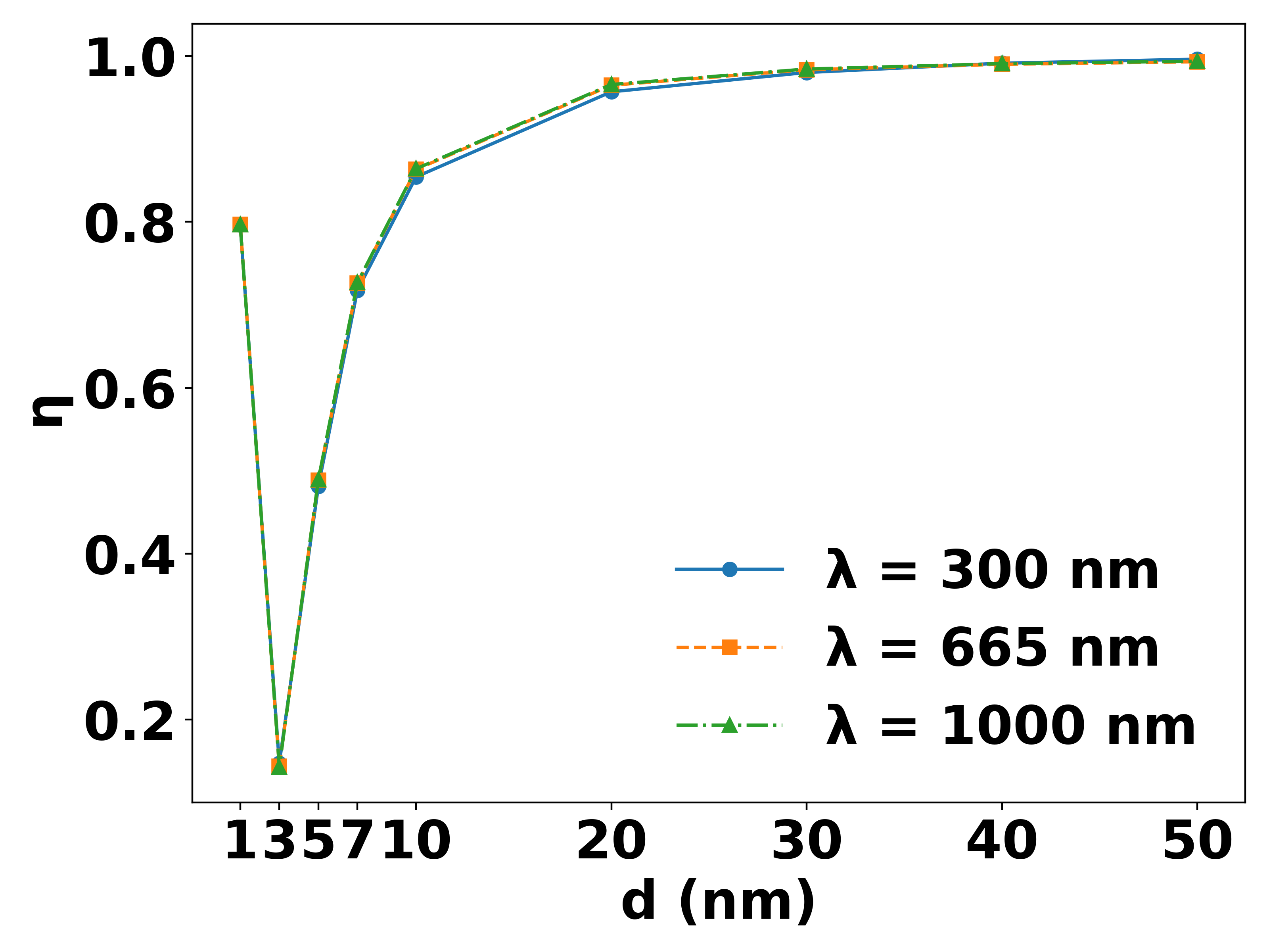
Example calibration/verification accuracy curve used to select a stable \(R_{x,\min}\) for BEM fitting.
Tip
The planar comparison is a validation workflow. For geometries without a closed-form reference (for example nanorods), reconstruction does not depend on this optional step.
References
U. Hohenester and A. Trugler, “MNPBEM - A Matlab toolbox for the simulation of plasmonic nanoparticles,” Computer Physics Communications 183 (2012) 370-381.
Liu, G., Wang, S. and Chen, H.T., 2026. MQED-QD: An Open-Source Package for Quantum Dynamics Simulation in Complex Dielectric Environments. Journal of Chemical Theory and Computation.