Spectral Density $J(\omega)$¶

Goal¶

In this tutorial you will learn how to:

Compute the spectral density $J_{\alpha\beta}(\omega)$ from pre-computed dyadic Green’s function (GF) data stored in HDF5 files.
Plot the resulting spectral density curves with customisable layout, labelling, and styling.

The spectral density links the electromagnetic environment (encoded in the imaginary part of the dyadic Green’s function) to the energy-transfer coupling between quantum emitters. It is defined as

\[J_{\alpha\beta}(\omega) = \frac{\omega^{2}}{\pi\,\hbar\,\varepsilon_{0}\,c^{2}}\; \boldsymbol{\mu}_{\alpha} \cdot \operatorname{Im}\!\bigl[\mathbf{G}(\mathbf{r}_{\alpha}, \mathbf{r}_{\beta};\omega)\bigr] \cdot \boldsymbol{\mu}_{\beta}\]

where $\boldsymbol{\mu}_{\alpha,\beta}$ are the transition dipole moments of the donor and acceptor, and the result is expressed in units of eV.

Prerequisites¶

A working MQED installation (see Getting Started).
A dyadic Green’s function HDF5 file produced by one of the GF tutorials (e.g. Dyadic Green’s Function via Sommerfeld Integrals). The file must contain the imaginary part of the GF together with the energy and position grids.

Quick start¶

Tip

If you have already run the Dyadic Green’s Function via Sommerfeld Integrals tutorial, the default configuration expects the output at ./data/gf_data.hdf5. Adjust the input_file path if your file is elsewhere.

Step 1 — Compute the spectral density Here we will continue with the GF data from the Dyadic Green’s Function via Sommerfeld Integrals tutorial and use the reference [Chuang2022] to compute the spectral density so that we could reproduce Figure 2C in that paper. We have put the dyadic Green’s function data at ./data/example/GF_data/Fresnel_GF_planar_Ag_height_1nm_Emin_0.10_Emax_6.00_359pts_Rx_33nm_34pts.hdf5 for user to follow along. The configuration file for this tutorial is configs/analysis/spec_dens_example.yaml, user can modify the input_file field to point to the above file:

input_file: "${oc.env:MQED_ROOT,./data}/example/GF_data/Fresnel_GF_planar_Ag_height_1nm_Emin_0.10_Emax_6.00_359pts_Rx_33nm_34pts.hdf5"

# --- Output ---
output_prefix: "spec_dens_${mu_D_debye}D_${mu_A_debye}D"

# --- Dipole moment magnitudes (Debye) ---
mu_D_debye: 10
mu_A_debye: 10

# --- Dipole orientations ---
# theta_deg: polar angle from z-axis (degrees).  Use 'magic' for the magic
#            angle θ ≈ 54.74° that averages orientational effects.
# phi_deg:   azimuthal angle in x-y plane (degrees).  Use 'magic' for
#            isotropic averaging.
orientations:
  donor:
    theta_deg: 90.0
    phi_deg: 0.0
  acceptor:
    theta_deg: 90.0
    phi_deg: 0.0

Here we set the both donor and acceptor dipoles to be x-oriented with a magnitude of 10 Debye. User can run the following command to compute the spectral density:

python -m mqed.analysis.spectral_density --config-name spec_dens_example

mqed_calc_spec_dens --config-name spec_dens_example

This reads the default configuration from configs/analysis/spec_dens_example.yaml, loads the GF data, computes the spectral density according to the specified parameters, and save the result in an HDF5 file. The output file spec_dens_10D_10D_Emin_0.10_Emax_6.00_359pts_height_1nm.hdf5 will be used in the next step for plotting the spectral density curve.

Step 2 — Plot the spectral density

python -m mqed.plotting.plot_spectral_density --config-name=plt_spec_dens_example

mqed_plot_spec_dens --config-name=plt_spec_dens_example

This reads the default configuration from configs/plots/plt_spec_dens_example.yaml, loads the spectral density HDF5 file produced in Step 1, and saves a publication-ready PNG figure. User can modify the configuration file to adjust the plot settings (e.g., axis labels, title, line styles) or override specific parameters from the command line.

The configuration looks like this:

 # configs/plots/plt_spec_dens_example.yaml

# --- Input ---
# Path to the spectral density HDF5 file produced by
# mqed.analysis.spectral_density.
input_file: "${oc.env:MQED_ROOT,./data}/example/spec_dens_data/spec_dens_10D_10D_Emin_0.10_Emax_6.00_359pts_height_1nm.hdf5"

# --- Font settings (following plot_pr.py conventions) ---
font:
  family: "Arial"
  labelsize: 18
  ticksize: 16
  legendsize: 14
  titlesize: 18
  labelweight: "bold"
  titleweight: "bold"

# --- Plot settings ---
plot_settings:
  # For separation-indexed layout: which Rx indices to plot (0-based)
  # Example: [0, 3] overlays the curves for Rx index 0 and Rx index 3.
  separation_indices: [0,3,33]
  separation_multipliers: [1.0,1.0,100]

  # For pair-indexed layout: which (α, β) pairs to plot
  # Each entry is [alpha, beta].  [0, 0] = self-term of emitter 0.
  # Example: [[0, 0], [0, 3]] overlays both pair-resolved curves.
  pair_indices:
    - [0, 0]
    - [0, 3]
  pair_multipliers: [1.0,1.0]

  # Labels
  # For separation layout, {Rx} is replaced by the Rx value in nm
  label_template: "Rx = {Rx:.1f} nm"
  xlabel: "Energy (eV)"
  ylabel: "$J(\\omega)$ (eV)"
  title: "Spectral Density $J(\\omega)$"

  # Axis scales: "linear" or "log"
  xscale: "linear"
  yscale: "linear"

  # Optional axis limits (null = auto)
  x_range_eV: [0,6]
  y_range: null

  # Style
  figsize: [8, 6]
  lw: 1.5
  dpi: 300
  grid: true

  # Output
  save_plot: true
  filename: "Spec_dens_drude.png"

The output figure will look like this: (identical to the reference [Chuang2022] Figure 2C up to axis labels and styling):

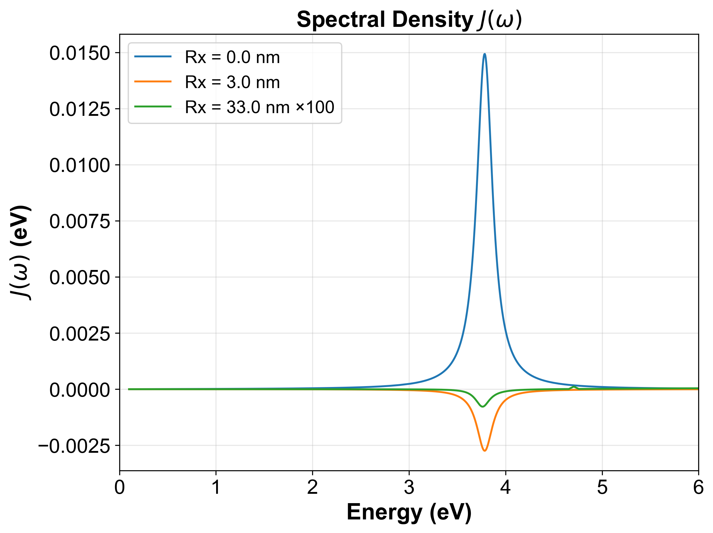
Note

Here our tutorial performs simulation on planar system with translation symmetry, so we only use the separation_indices to specify which curves to plot because the GF data is in separation-indexed layout.

In the future, we will add examples with pair_indices for systems without translation symmetry, where the GF data is in pair-indexed layout and requires specifying emitter pairs to plot.

Configuration reference — analysis¶

The analysis step is configured by configs/analysis/spectral_density.yaml. A minimal version looks like:

# configs/analysis/spectral_density.yaml

input_file:  '${oc.env:MQED_ROOT,./data}/gf_data.hdf5'
output_file: 'spectral_density.hdf5'

orientations:
  donor:
    theta_deg: 90.0
    phi_deg:   0.0
  acceptor:
    theta_deg: 90.0
    phi_deg:   0.0

Analysis parameters¶
Parameter	Default	Description
`input_file`	`./data/gf_data.hdf5`	Path to the GF HDF5 file (supports `${oc.env:MQED_ROOT}` interpolation).
`output_file`	`spectral_density.hdf5`	Output HDF5 file for the computed spectral density.
`orientations.donor.theta_deg`	`90.0`	Polar angle $\theta$ (degrees) of the donor transition dipole moment.
`orientations.donor.phi_deg`	`0.0`	Azimuthal angle $\phi$ (degrees) of the donor transition dipole moment.
`orientations.acceptor.theta_deg`	`90.0`	Polar angle $\theta$ (degrees) of the acceptor transition dipole moment.
`orientations.acceptor.phi_deg`	`0.0`	Azimuthal angle $\phi$ (degrees) of the acceptor transition dipole moment.

Tip

You can specify the magic angle orientation ($\theta \approx 54.74°$) by using the keyword magic in place of a numeric value in any theta_deg or phi_deg field.

Specifying dipole orientations¶

The orientation of each transition dipole is given in spherical coordinates $(\theta, \phi)$. Common choices:

x-oriented dipole — theta_deg: 90, phi_deg: 0
y-oriented dipole — theta_deg: 90, phi_deg: 90
z-oriented dipole — theta_deg: 0, phi_deg: 0
Magic angle — theta_deg: magic (≈ 54.74°, isotropic average)

To override the orientations from the command line:

python -m mqed.analysis.spectral_density \
    orientations.donor.theta_deg=0 \
    orientations.acceptor.theta_deg=0

This sets both donor and acceptor dipoles to the z-direction.

Using a custom configuration file¶

You can point Hydra at a different configuration directory or override the config name (Similar in tutorial Dyadic Green’s Function via Sommerfeld Integrals):

mqed_plot_spec_dens \
    --config-path /absolute/path/to/my_configs \
    --config-name my_spectral_density

Or override individual values via the command line:

mqed_plot_spec_dens \
    --config-path /absolute/path/to/my_configs \
    --config-name my_spectral_density

Configuration reference — plotting¶

The plotting step is configured by configs/plots/spectral_density.yaml. A minimal version looks like:

# configs/plots/spectral_density.yaml

input_file: '${oc.env:MQED_ROOT,./outputs}/spectral_density/spectral_density.hdf5'

font:
  family:       Arial
  labelsize:    18
  ticksize:     16
  legendsize:   14
  titlesize:    18
  labelweight:  bold
  titleweight:  bold

plot_settings:
  separation_indices: [0]
  pair_indices:       [[0, 0]]
  label_template:     'Rx = {Rx:.1f} nm'
  xlabel:             'Energy (eV)'
  ylabel:             'J (eV)'
  title:              'Spectral Density'
  xscale:             linear
  yscale:             linear
  figsize:            [8, 5]
  lw:                 1.5
  dpi:                300
  grid:               true
  save_plot:          true
  filename:           'spectral_density.png'

Plotting parameters¶
Parameter	Default	Description
`input_file`	(see YAML)	Path to the spectral density HDF5 file.
`font.family`	`Arial`	Matplotlib font family.
`font.labelsize`	`18`	Font size for axis labels.
`font.ticksize`	`16`	Font size for tick labels.
`font.legendsize`	`14`	Font size for the legend.
`font.titlesize`	`18`	Font size for the plot title.
`font.labelweight`	`bold`	Font weight for axis labels.
`font.titleweight`	`bold`	Font weight for the plot title.
`plot_settings.separation_indices`	`[0]`	List of separation (Rx) indices to plot when using the separation-indexed GF layout.
`plot_settings.pair_indices`	`[[0, 0]]`	List of emitter-pair index pairs `[i, j]` to plot when using the pair-indexed GF layout.
`plot_settings.label_template`	`Rx = {Rx:.1f} nm`	Python format string for the legend label. `{Rx}` is replaced by the Rx value in nanometres.
`plot_settings.xlabel`	`Energy (eV)`	Label for the x-axis.
`plot_settings.ylabel`	`J (eV)`	Label for the y-axis.
`plot_settings.title`	`Spectral Density`	Plot title.
`plot_settings.xscale`	`linear`	Scale for the x-axis (`linear` or `log`).
`plot_settings.yscale`	`linear`	Scale for the y-axis (`linear` or `log`).
`plot_settings.figsize`	`[8, 5]`	Figure size in inches `[width, height]`.
`plot_settings.lw`	`1.5`	Line width for the plotted curves.
`plot_settings.dpi`	`300`	Resolution of the saved figure.
`plot_settings.grid`	`true`	Whether to display a grid on the plot.
`plot_settings.save_plot`	`true`	Whether to save the figure to disk.
`plot_settings.filename`	`spectral_density.png`	Filename for the saved figure.

Customising the plot from the command line¶

Override any plotting parameter via Hydra:

python -m mqed.plotting.plot_spectral_density \
    plot_settings.xscale=log \
    plot_settings.yscale=log \
    plot_settings.title='Log-scale Spectral Density' \
    plot_settings.filename=spectral_density_log.png

Expected output¶

After running Step 1 (analysis), the output HDF5 file (spectral_density.hdf5) contains:

J_eV — the spectral density array in eV. The shape depends on the GF layout:
- Separation layout [K, M]: K separation indices, M energy points.
- Pair layout [N, N, M]: all emitter pairs for N emitters over M energy points.
energy_eV — the energy grid in eV.
Rx_nm (separation layout only) — the donor–acceptor separations in nanometres.

After running Step 2 (plotting), you will find a PNG file (default: spectral_density.png) showing $J_{\alpha\beta}(\omega)$ versus energy.

Using the output in downstream analyses¶

The spectral density is a key input for quantum-dynamics simulations. You can load it in your own scripts:

import h5py
import numpy as np

with h5py.File('spectral_density.hdf5', 'r') as f:
    J_eV     = np.array(f['J_eV'])
    energy_eV = np.array(f['energy_eV'])

# Use J_eV and energy_eV in your quantum-dynamics workflow
# e.g., as input to the Lindblad master equation solver

References¶

[Chuang2022] (1,2)

Chuang et al., “Chuang, Y.T., Lee, M.W. and Hsu, L.Y., 2022. Tavis-Cummings model revisited: A perspective from macroscopic quantum electrodynamics. Frontiers in Physics, 10, p.980167.”

Spectral Density \(J(\omega)\)¶

Goal¶

Prerequisites¶

Quick start¶

Configuration reference — analysis¶

Specifying dipole orientations¶

Using a custom configuration file¶

Configuration reference — plotting¶

Customising the plot from the command line¶

Expected output¶

Using the output in downstream analyses¶

References¶