Dyadic Green’s Function via Sommerfeld Integrals

Goal

In this tutorial you will compute the dyadic Green’s function \(\overleftrightarrow{G}(\mathbf{r}_D, \mathbf{r}_A, \omega)\) for a two-layer planar system (vacuum above a semi-infinite substrate) using the Fresnel-coefficient / Sommerfeld-integral method implemented in MQED-QD.

By the end you will know how to:

• run the mqed_GF_Sommerfeld command with default and custom parameters,

• specify single-frequency, multi-frequency (list), and swept-frequency (dict) inputs (including segmented nonuniform windows),

• choose dielectric models from YAML (excel, constant, Drude, Drude-Lorentz),

• accelerate multi-frequency sweeps with joblib (multicore) or MPI (cluster) parallelism,

• locate and interpret the HDF5 output file.

See also

Two-Layer Planar Geometry for the mathematical derivation of the Sommerfeld integrals and Fresnel reflection coefficients used by this solver.

Prerequisites

Make sure you have installed the package and activated the environment as described in Installation.

Quick start

Example 1: Single frequency simulation with 100 molecular aggregates

Here we give an example of how to simulate dyadic Green’s function for a single energy point which will be used for quantum dynamics of 100 molecular aggregates with intermolecular distance d = 3 nm at a height of z = 5 nm above the silver surface (which is specified by zD: 5.0e-9 and zA: 5.0e-9 in the below). In this setup, we will need 301 horizontal distance points from x = 0 nm to x = 300 nm to cover the interaction between all pairs of aggregates. (x = 0 nm corresponds to the position of donor and outputs the self-interaction of the aggregate, i.e, decay rate.) The corresponding configuration file is configs/Dyadic_GF/GF_Sommerfeld_example_single_freq.yaml and the command to run is:

mqed_GF_Sommerfeld --config-name=GF_Sommerfeld_example_single_freq

Here is the configuration file with annotations:

# ── Material ────────────────────────────────────────────
material:
  source_type: excel          # excel, constant, Drude, Drude-Lorentz
  constant_value: 9.0+0.0j   # used only when source_type = 'constant'
  excel_config:
    filepath: "DielectricFunction/dielectric function.xlsx"
    sheet_name: "Ag_BEM"
  drude_config:               # used only when source_type = 'Drude'
    eps_inf: 1.0
    omega_p_eV: 9.01          # or omega_p_rad_s
    gamma_eV: 0.048           # or gamma_rad_s
  drude_lorentz_config:       # used only when source_type = 'Drude-Lorentz'
    eps_inf: 1.0
    omega_p_eV: 9.01
    gamma_eV: 0.048
    oscillators:
      - strength: 0.85
        omega_0_eV: 3.8       # or omega_0_rad_s
        gamma_eV: 0.25        # or gamma_rad_s

# ── Simulation ──────────────────────────────────────────
simulation:
  material: "Ag"             # label used in the output filename
  spectral_param: "energy_eV"  # 'energy_eV' or 'wavelength_nm'

  energy_eV: 1.864                 # single value, list, dict, or piecewise segments


  wavelength_nm:             # same three formats as energy_eV
    min: 500.0
    max: 500.0
    points: 1

  position:
    zD: 5.0e-9              # donor height above surface (m)
    zD_nm: 5                # donor height label for filename (nm)
    zA: 5.0e-9              # acceptor height above surface (m)
    Rx_nm:                  # horizontal donor–acceptor distances
      start: 0.0
      stop: 300.0
      points: 301           # 0, 1, 2, …, 300 nm

This file specifies a single frequency point at 1.864 eV.

After running the command, user can observe the progress bar in the terminal:

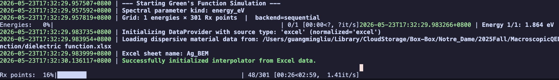
Running progress bar in the terminal.

After the simulation finishes, a success message is printed to the terminal and user can find the output HDF5 file in the specified output directory. The output file contains the computed dyadic Green’s function data and related parameters, which can be used for downstream analyses such as field enhancement calculations or quantum dynamics simulations.

Specifying the emitter frequency

You can override any configuration key on the command line using Hydra syntax. (See the YAML configurations in the below.)

Single energy

mqed_GF_Sommerfeld simulation.energy_eV=1.864

List of energies

mqed_GF_Sommerfeld simulation.energy_eV=[1.5,1.8,2.0]

Swept range (dict input)

mqed_GF_Sommerfeld simulation.energy_eV.min=1.0 \
    simulation.energy_eV.max=2.0 \
    simulation.energy_eV.points=11

This generates 11 linearly spaced energies from 1.0 to 2.0 eV.

Segmented nonuniform sweep (piecewise ranges)

mqed_GF_Sommerfeld \
    simulation.energy_eV.segments[0].min=0.0 \
    simulation.energy_eV.segments[0].max=3.0 \
    simulation.energy_eV.segments[0].points=21 \
    simulation.energy_eV.segments[1].min=3.0 \
    simulation.energy_eV.segments[1].max=4.5 \
    simulation.energy_eV.segments[1].points=301 \
    simulation.energy_eV.segments[2].min=4.5 \
    simulation.energy_eV.segments[2].max=6.0 \
    simulation.energy_eV.segments[2].points=21

This is useful when the spectrum is mostly flat away from resonance and needs fine resolution only near the plasmonic window.

Choosing the dielectric model

The dielectric source is selected by material.source_type:

• excel: interpolate from the configured Excel sheet

• constant: use a fixed complex permittivity (Useful for non-dispersive material)

• Drude: use the Drude model

• Drude-Lorentz: use Drude + Lorentz oscillators

Examples:

# Constant epsilon
mqed_GF_Sommerfeld material.source_type=constant material.constant_value="9.0+0.2j"

# Drude model with eV parameters
mqed_GF_Sommerfeld material.source_type=Drude \
    material.drude_config.eps_inf=1.0 \
    material.drude_config.omega_p_eV=9.01 \
    material.drude_config.gamma_eV=0.048

# Drude-Lorentz model with two oscillators
mqed_GF_Sommerfeld material.source_type=Drude-Lorentz \
    material.drude_lorentz_config.eps_inf=1.0 \
    material.drude_lorentz_config.omega_p_eV=9.01 \
    material.drude_lorentz_config.gamma_eV=0.048 \
    material.drude_lorentz_config.oscillators[0].strength=0.85 \
    material.drude_lorentz_config.oscillators[0].omega_0_eV=3.8 \
    material.drude_lorentz_config.oscillators[0].gamma_eV=0.25 \
    material.drude_lorentz_config.oscillators[1].strength=0.20 \
    material.drude_lorentz_config.oscillators[1].omega_0_eV=4.9 \
    material.drude_lorentz_config.oscillators[1].gamma_eV=0.35

Note

For each frequency-like model parameter, provide exactly one unit key: *_eV or *_rad_s.

Tip

You can use wavelength instead of energy by setting simulation.spectral_param=wavelength_nm and providing simulation.wavelength_nm values in the same single / list / dict format. We provide this feature for some users who prefer wavelength in their research. However, our simulation example will focus on eV. User needs to verify the physical accuracy when using wavelength in their simulation.

Using a custom configuration file

Every MQED command loads its default YAML from the configs/ directory. Hydra provides two flags that let you swap the entire configuration file without editing code:

Use a different YAML in the same config directory If we are trying to simulate multiple different parameters and want to keep track of our previous simulation configuration, we naturally want to use different configuration files which is significantly easier than modify the single hydra file every time in a new simulation. Luckily, Hydra helps us to achieve this by telling it the --config-name and --config-dir which specify the path and name of YAML file where we put in the project subdirectory.

mqed_GF_Sommerfeld --config-name=my_GF

This loads configs/Dyadic_GF/my_GF.yaml instead of the default GF_Sommerfeld.yaml. Your custom file my_GF.yaml must live in the same configs/Dyadic_GF/ directory. User need to manually create my_GF.yaml inside configs/Dyadic_GF.

Use a YAML from an arbitrary directory

mqed_GF_Sommerfeld --config-dir=/path/to/my/configs --config-name=my_GF

This tells Hydra to look for my_GF.yaml in /path/to/my/configs/ instead of the default config directory configs/Dyadic_GF/. This helps user to seperate individual simulation directory from our project directory.

Tip

You can combine --config-name (or --config-dir) with individual parameter overrides:

mqed_GF_Sommerfeld --config-name=my_GF simulation.energy_eV=2.0

Parallel execution

When computing the Green’s function over many frequencies (e.g. a 200-point spectral density sweep), the sequential loop can take tens of minutes. Because each energy point is completely independent, the frequency axis can be parallelized with no inter-worker communication.

MQED-QD supports two parallel backends, selectable via the parallel configuration group.

Joblib (shared-memory multiprocessing)

Best for laptops and single-node workstations. Uses Python’s multiprocessing under the hood via joblib.

# Use all available CPU cores
mqed_GF_Sommerfeld \
    simulation.energy_eV='{min: 0.5, max: 4.0, points: 200}' \
    parallel.backend=joblib

# Limit to 4 workers
mqed_GF_Sommerfeld \
    simulation.energy_eV='{min: 0.5, max: 4.0, points: 200}' \
    parallel.backend=joblib parallel.n_jobs=4

Setting parallel.n_jobs=-1 (the default) uses all available cores. We recommend user to set parallel.n_jobs=-2 to leave at least one core for their computer to avoid accidental shutdown.

Tip

On a machine with 8 cores, a 200-energy sweep that takes ~30 min sequentially will finish in ~4 min with parallel.backend=joblib.

MPI (distributed parallelism)

Best for HPC clusters with multi-node allocation. Requires mpi4py and an MPI runtime (e.g. OpenMPI or MPICH).

Auto-launch mode (default) — the script detects it is not inside an MPI communicator and re-launches itself under mpiexec:

mqed_GF_Sommerfeld \
    simulation.energy_eV='{min: 0.5, max: 4.0, points: 200}' \
    parallel.backend=mpi parallel.mpi_nproc=16

Manual launch — submit from a job scheduler (SLURM, PBS, etc.) with mpi_auto_launch=false:

# Inside a SGE job script, for example:
qsub -v GF_CONFIG_NAME=GF_Sommerfeld_custom\
mqed/Dyadic_GF/gf_sommerfeld_single_job.sh
# This script will use the specified config 'GF_Sommerfeld_custom.yaml'
# inside configs/Dyadic_GF/ and run with MPI parallelism.

Energy points are scattered round-robin across MPI ranks. Only rank 0 writes the final HDF5 file. User can adjust the number of ranks with parallel.mpi_nproc. User can also choose their own YAML file with the GF_CONFIG_NAME environment variable (e.g. GF_Sommerfeld_custom.yaml) when submitting the job script.

Parallel configuration reference

Parameter	Description	Default
parallel.backend	Execution mode: sequential, joblib, or mpi	sequential
parallel.n_jobs	Number of joblib workers (-1 = all cores)	-1
parallel.mpi_nproc	Number of MPI ranks for auto-launch	4
parallel.mpi_auto_launch	Re-launch under mpiexec automatically	true
parallel.mpi_exec	Path to MPI launcher binary	mpiexec

Note

Users running on the HPC cluster with SLURM scheduler may need to modify the job script to fit their cluster environment.

Example 2: Multiple frequencies simulation for Spectral Density Here we will use the example configuration file configs/Dyadic_GF/GF_Sommerfeld_example_multi_freq.yaml to compute the Green’s function for a range of frequencies which will be used for calculating the spectral density in the next tutorial. We will use parameters from the previous literature [Chuang2022tavis] to model the dielectric function of silver with a Drude model. The parameter used in modified Drude model is: \(\epsilon_{Ag}(\omega) = \epsilon_{\infty,Ag} - \frac{\omega_{p,Ag}^2}{\omega^2 + i\gamma_{p,Ag}\omega}\) where \(\epsilon_{\infty,Ag}=5.3\), \(\omega_{p,Ag}=9.5 eV\), and \(\gamma_{p,Ag}=0.2 eV\) and the YAML file is shown below with annotations:

material:
   source_type: drude

  # --- Settings for a CONSTANT material ---
  # This value is used only if source_type is 'constant'
  constant_value: 9.0+0.0j # Example for a non-dispersive material

  # --- Settings for an EXCEL-based material ---
  # This section is used only if source_type is 'excel'
  excel_config:
    filepath: "DielectricFunction/dielectric function.xlsx"
    sheet_name: "Ag_BEM"

  drude_config:
    eps_inf: 5.3
    omega_p_eV: 9.5
    gamma_eV: 0.2

  drude_lorentz_config:
    eps_inf: 1.0
    omega_p_eV: 9.01
    gamma_eV: 0.048
    oscillators:
      - strength: 0.85
        omega_0_eV: 3.8
        gamma_eV: 0.25
      - strength: 0.20
        omega_0_eV: 4.9
        gamma_eV: 0.35

simulation:
  material: "Ag" # Material surface
  spectral_param: "energy_eV" # Choose between 'wavelength_nm' or 'energy_eV'

  energy_eV:
    segments:
      - min: 0.1
        max: 3.0
        points: 29
      - min: 3.0
        max: 4.5
        points: 300
      - min: 4.5
        max: 6.0
        points: 30

  wavelength_nm: # same usage as energy_eV
    min: 500.0
    max: 500.0
    points: 1
  position:
    zD: 1.0e-9
    zD_nm: 1 # Key for name
    zA: 1.0e-9
    Rx_nm: # New section to define the range of horizontal distances
      start: 0.0
      stop: 33.0
      points: 34 # This will give you points 1, 2, 3, ...

Here we specify a segmented energy sweep with 29 points from 0.1 to 3.0 eV, 300 points from 3.0 to 4.5 eV, and 30 points from 4.5 to 6.0 eV to capture the plasmonic resonance of silver planar surface (The resonant frequency is around 3.8 eV so that we choose finer energy points around that region. For other energy grids, we use larger segments due to ‘spectrally-flat’, i.e, the value changes little with frequencies in this region.).

In the terminal, user could run command

GF_CONFIG_NAME=GF_Sommerfeld_example_multi_freq bash mqed/Dyadic_GF/gf_sommerfeld_single_job.sh

to run the simulation with MPI parallelism on their own laptop (Not recommended in general, but for this small simulation, it is acceptable). This script assumes an MPI runtime is installed and the mqed conda environment is available. In the HPC cluster, user can submit the job script with

qsub -v GF_CONFIG_NAME=GF_Sommerfeld_example_multi_freq mqed/Dyadic_GF/gf_sommerfeld_single_job.sh

to run the simulation with MPI parallelism.

User can observe the following information in the terminal:

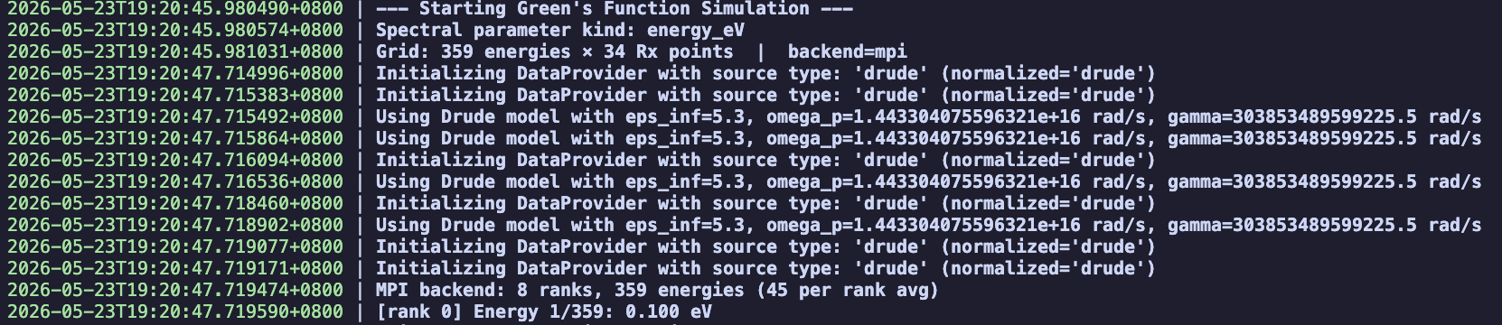
The output file will be used to calculate spectral density in our tutorial: Spectral Density J(\omega).

Configuration reference

Key parameters at a glance

Parameter	Description	Default
material.source_type	Source of the dielectric function (excel, constant, Drude, Drude-Lorentz)	excel
simulation.spectral_param	Which spectral unit to use (energy_eV or wavelength_nm)	energy_eV
simulation.position.zD	Donor height above the surface in meters	5.0e-9
simulation.position.zA	Acceptor height above the surface in meters	5.0e-9
simulation.position.Rx_nm	Horizontal distance grid (start, stop, points) in nm	0 – 300 nm, 301 pts
simulation.integration.epsabs	Absolute tolerance for Sommerfeld quadrature	1.0e-10
simulation.integration.limit	Maximum sub-intervals for adaptive quadrature	400

Warning

Before running any script on HPC cluster, user need to install MQED-QD package in the cluster environment and make sure the path to the package is correct in the job script. If user is running the Slurm script, please modify gf_sommerfeld_single_job.sh according to the guidance.

Expected output

After the simulation finishes, a success message is printed to the terminal (and to the Hydra log file outputs/Dyadic_GF_Sommerfeld/.../Dyadic_GF_Sommerfeld.log):

2025-10-24 11:40:02.818 | SUCCESS | mqed.Dyadic_GF.main:run_simulation:114
- Simulation complete. Output saved to:
  /.../MacroscopicQED/outputs/Dyadic_GF_Sommerfeld/Y-M-D/H-M-S/YOUR_NAME.hdf5

The output is an HDF5 file that stores:

• the 9-component dyadic Green’s function (total and vacuum) as 4-D complex arrays of shape [nE, nR, 3, 3],

• the energy grid (energy_eV),

• the horizontal distance grid (Rx_nm),

• the donor and acceptor heights (zD, zA).

Using the output in downstream analyses

Many MQED-QD workflows read a cached Green’s function file as their input. The recommended workflow is:

1. Create a cache directory under the project root (if it does not exist):

   mkdir -p data/GF_cache
   

2. Copy (or symlink) the HDF5 result into the cache:

   cp outputs/Dyadic_GF_Sommerfeld/<date>/<time>/YOUR_NAME.hdf5 \
      data/GF_cache/
   

3. Update the greens.h5_path or input_file key in the downstream configuration to point to this cached file.

See also

• Field Enhancement – compute the field enhancement using the Green’s function produced here.

• Quantum Dynamics – run Lindblad or NHSE dynamics with this Green’s function as input.

• Spectral Density J(\omega) – compute the spectral density from this Green’s function.

References

[Chuang2022tavis]

Chuang et al., “Chuang, Y.T., Lee, M.W. and Hsu, L.Y., 2022. Tavis-Cummings model revisited: A perspective from macroscopic quantum electrodynamics. Frontiers in Physics, 10, p.980167.”