Mie Green’s Function for Spherical Cavities¶

Goal¶

This tutorial shows how to run the generalized Mie Green-function workflow for a spherical core-shell cavity and then use the result in the spectral-density pipeline. It focuses on the verified scan workflow used by the bundled configs/Dyadic_GF/GF_Mie.yaml example.

By the end you will know how to:

run the core-shell spherical-cavity config,
understand source_position_nm versus position.Rx_nm in scan layout,
inspect the shared HDF5 output schema,
compute and plot spectral density curves at 0, 2, and 20 nm observer offsets,
launch a many-frequency job with the SGE/MPI helper script.

Important limitation¶

The Mie implementation is experimental and should still be benchmarked against literature or independent codes for each new physical regime. The current core-shell scan path is intended for source and observer points inside the core/cavity. Shell-region observation points currently return zero structure terms with a warning.

Symmetry-reduced emitter rings¶

For an equally spaced emitter ring around a concentric sphere, with dipole orientations generated by simulation.emitter_ring, the projected scalar coupling matrix is circulant. The opt-in configs/Dyadic_GF/GF_sphere_ring_circulant_example.yaml configuration uses output.layout: ring_circulant to compute and store only one cyclic row per energy, with shape (M, N). The full scalar matrix is reconstructed as G[m, i, j] = row[m, (j-i) mod N] by supported analysis and dynamics tools.

This reduction does not assert a universal Tavis-Cummings model and does not store Cartesian dyadics. Keep output.layout: pair (as in GF_sphere_example.yaml) for arbitrary emitter positions, incompatible orientations, or consumers that require the full (M, N, N, 3, 3) tensor.

Quick run¶

Run the bundled annotated config:

mqed_GF_Mie --config-name GF_Mie

The config is located at:

configs/Dyadic_GF/GF_Mie.yaml

It computes a core-shell spherical cavity with radii [160, 60] nm and an Aluminum Drude shell. The expected filename is:

mie_shell_cavity_scan_Emin_0.10_Emax_8.00_122pts_Rx_20nm_3pts.hdf5

The exact directory is the active Hydra run directory.

For a fast smoke test, reduce the energy grid from the command line:

mqed_GF_Mie \
  --config-name GF_Mie \
  parallel.backend=sequential \
  simulation.energy_eV='[1.8]' \
  simulation.position.Rx_nm='[0.0,2.0,20.0]'

Geometry and regions¶

The core-shell convention is:

simulation:
  geometry:
    boundary: coreshell
    radii_nm: [160.0, 60.0]

For this example:

region 0 is the exterior, r >= 160 nm,
region 1 is the shell, 60 <= r < 160 nm,
region 2 is the core/cavity, r < 60 nm.

The geometry is shown schematically below:

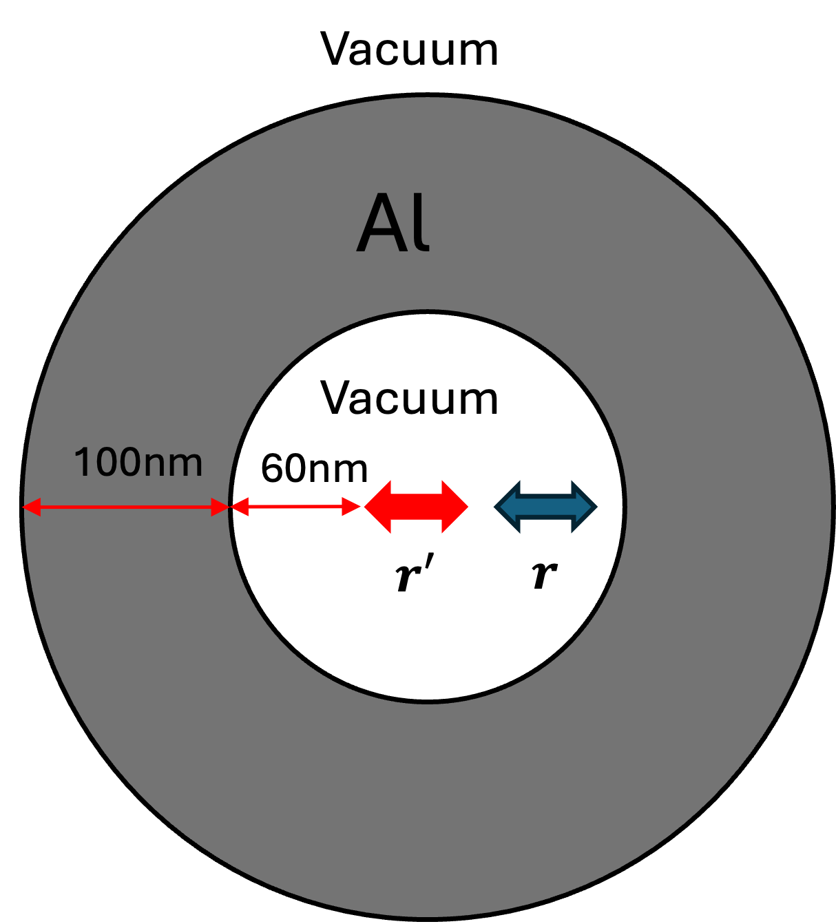
../_images/visualization_spherical_cavity.png — Core-shell spherical cavity with 160 nm outer radius and 60 nm inner radius. The source is at the center and the observers are at 0, 2, and 20 nm offsets.¶

The bundled scan points 0, 2, 20 nm all remain inside the core/cavity.

Scan layout: source and observer positions¶

The default Mie config uses:

simulation:
  source_position_nm: [0.0, 0.0, 0.0]
  position:
    Rx_nm: [0.0, 2.0, 20.0]
output:
  layout: scan

In scan layout:

source_position_nm is the fixed source/donor dipole position.
position.Rx_nm gives observer/acceptor x-offsets relative to that source.
The driver computes G(observer, source) for each observer and energy.

With the settings above, the observer positions are:

[0,  0, 0] nm
[2,  0, 0] nm
[20, 0, 0] nm

and the source position is always [0, 0, 0] nm.

Note

Do not add emitter_positions_nm to a scan-layout config. That key is used by output.layout: pair to compute all tensors G(r_observer_i, r_source_j) for a list of emitters.

Energy grid¶

The default example uses three energy segments:

simulation:
  spectral_param: energy_eV
  energy_eV:
    segments:
      - min: 0.1
        max: 6.0
        points: 59
      - min: 6.01
        max: 6.5
        points: 49
      - min: 6.6
        max: 8.0
        points: 14

This gives 122 energy points. Segmented grids are useful when a narrow spectral window needs more resolution than the rest of the spectrum.

Output schema¶

The Mie driver writes the shared scan HDF5 layout:

green_function_total[M, P, 3, 3]
green_function_vacuum[M, P, 3, 3]
green_function_structure[M, P, 3, 3]
energy_eV[M]
observer_positions_nm[P, 3]
source_position_nm[3]
observer_distances_nm[P]       # after spectral-density analysis
gf_layout = "scan"

For the bundled config, M = 122 and P = 3. Compatibility aliases such as G_total and G_structure are also present for older scripts.

Compute spectral density¶

After the Mie HDF5 file has been produced, compute spectral density with:

mqed_calc_spec_dens \
  --config-name spectral_density \
  input_file=/path/to/mie_shell_cavity_scan_Emin_0.10_Emax_8.00_122pts_Rx_20nm_3pts.hdf5 \
  output_prefix=spec_dens_mie_scan \
  mu_D_debye=1 \
  mu_A_debye=1

The spectral-density output preserves the scan metadata:

J_eV[P, M]
observer_positions_nm[P, 3]
source_position_nm[3]
observer_distances_nm[P]
gf_layout = "scan"

For this example, observer_distances_nm is [0, 2, 20].

Plot the scan curves¶

Use the spectral-density plotting command and choose curves by physical scan distance:

mqed_plot_spec_dens \
  --config-name plt_spec_dens_direct_sg \
  curves=[] \
  input_file=/path/to/spec_dens_mie_scan_Emin_0.10_Emax_8.00_122pts_height_0nm.hdf5 \
  plot_settings.scan_distance_values_nm='[0,2,20]' \
  plot_settings.scan_label_template='R = {distance_nm:.0f} nm' \
  plot_settings.filename=Spec_dens_mie_scan.png

The curves=[] override disables the comparison-file list in the bundled N-layer plotting example so the command uses the single Mie input_file. scan_distance_values_nm is preferred for Mie scan output because it selects curves by physical observer-source distance rather than by array index.

The result should look like: (See literature [Chuang2022sphere])

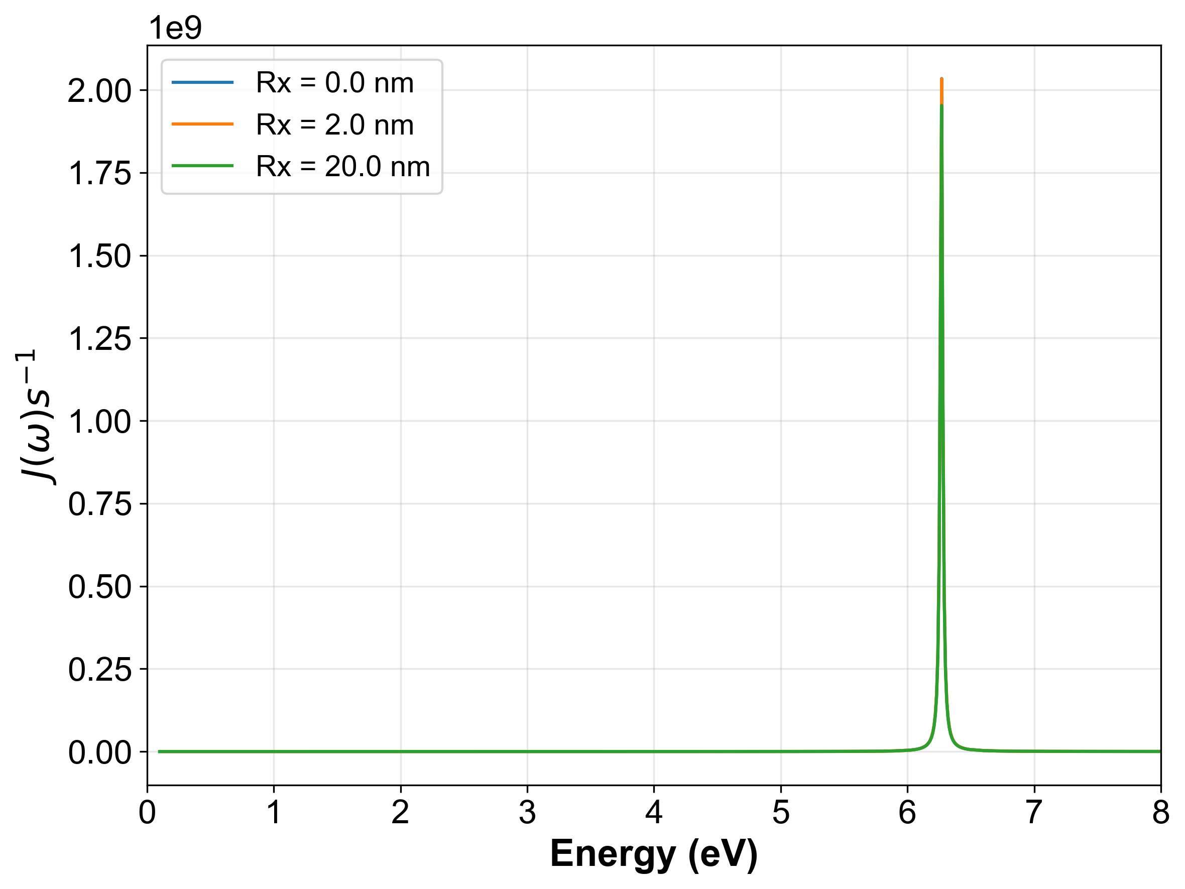
../_images/Spec_dens_Yiting_spherical.png — Spectral density for a spherical cavity with 0, 2, and 20 nm observer offsets.¶

HPC launcher¶

For the full many-frequency run, submit the Mie helper script:

qsub mqed/Dyadic_GF/gf_mie_single_job.sh

To use a personal config (put it inside configs/Dyadic_GF/), set the environment variable GF_CONFIG_NAME:

qsub -v GF_CONFIG_NAME=Your_CONFIG_NAME \
     mqed/Dyadic_GF/gf_mie_single_job.sh

You can dry-run the exact command without starting the calculation:

DRY_RUN=1 GF_CONFIG_NAME=GF_Mie bash mqed/Dyadic_GF/gf_mie_single_job.sh

Common mistakes¶

Confusing scan and pair layouts: scan has one fixed source and many observers; pair computes all emitter-emitter tensor pairs.
Putting observers in the shell: for the current core-shell scan path, keep observer radii below the 60 nm core radius unless you intentionally want warning/zero-structure placeholders.
Expecting translational symmetry: unlike N-layer Rx output, Mie scan positions are explicit Cartesian positions in a spherical geometry.
Skipping benchmarks: use the Mie results as a workflow foundation, then validate against literature or an independent implementation before drawing physical conclusions.

Next steps¶

Spectral Density J(\omega) for detailed analysis and plotting options.
N-Layer Dyadic Green’s Function Workflow for planar multilayer systems.
Dyadic Green’s Function via Sommerfeld Integrals for the two-layer planar baseline.

References¶

[Chuang2022sphere]

Chuang et al., “Chuang, Y.T., Lee, M.W. and Hsu, L.Y., 2022. Tavis-Cummings model revisited: A perspective from macroscopic quantum electrodynamics. Frontiers in Physics, 10, p.980167.”